UPDATE: more edits & enhancements for clarity made at 3:35 CDT, June 17, 2010.

I’ve returned to the issue of determining to what extent the Pacific Decadal Oscillation (PDO) can at least partly explain global average temperature variations, including warming, during the 20th Century. We tried publishing a paper on this over a year ago and were immediately and swiftly rejected in a matter of days by a single (!) reviewer.

Here I use a simple forcing-feedback model, combined with satellite estimates of cloud changes caused by the PDO, to demonstrate the ability of the model to explain the temperature variations. This time, though, I am going to use Jim Hansen’s (GISS) record of yearly radiative forcings of the global climate system since 1900 to demonstrate more convincingly the importance of the PDO…not only for explaining the global temperature record of the past, but for the estimation of the sensitivity of the climate system and thus project the amount of future global warming (er, I mean climate change).

What follows is not meant to be publishable in a peer-reviewed paper. It is to keep the public informed, to stimulate discussion, to provide additional support for the claims in my latest book, and to help me better understand what I know at this point in my research, what I don’t know, and what direction I should go next.

The Simple Climate Model
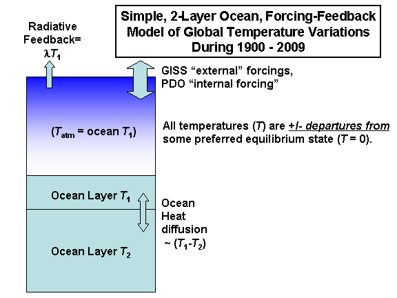
I’m still using a simple forcing feedback-model of temperature variations, but have found that more than a single ocean layer is required to mimic both the faster time scales (e.g. 5-year) temperature fluctuations, while allowing a slower temperature response on multi-decadal time scales as heat diffuses from the upper ocean to the deeper ocean. The following diagram shows the main components of the model.

For forcing, I am assuming the GISS record of yearly-average forcing, the values of which I have plotted for the period since 1900 in the following graph:

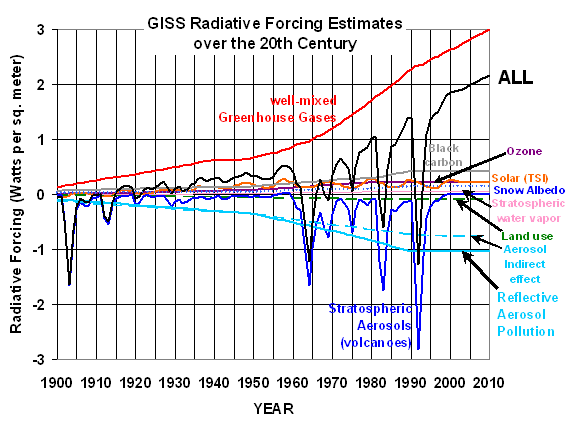
I will simply assume these forcings are correct, and will show what happens in the model when I use: (1) all the GISS forcings together; (2) all GISS forcings except tropospheric aerosols, and (3) all the GISS forcings, but replacing the tropospheric aerosols with the satellite-derived PDO forcings.

Internal Radiative Forcing from the PDO
As readers here are well aware, I believe that there are internal modes of climate variability which can cause “internal radiative forcing” of the climate system. These would most easily be explained as circulation-induced changes in cloud cover. My leading candidate for this mechanism continues to be the Pacific Decadal Oscillation.

We have estimated the radiative forcing associated with the PDO by comparing yearly global averages of them to similar averages of CERES radiative flux variations over the Terra CERES period of record, 2000-2009. But since the CERES-measured radiative imbalances are a combination of forcing and feedback, we must remove an estimate of the feedback to get at the PDO forcing. [This step is completely consistent with, and analogous to, previous investigators removing known radiative forcings from climate model output in order to estimate feedbacks in those models].

Our new JGR paper (still awaiting publication) shows evidence that, for year-to-year climate variability at least, net feedback is about 6 Watts per sq. meter per degree C. After removal of the feedback component with our AMSU-based tropospheric temperature anomalies, the resulting relationship between yearly-running 3-year average PDO index versus radiative forcing looks like this:

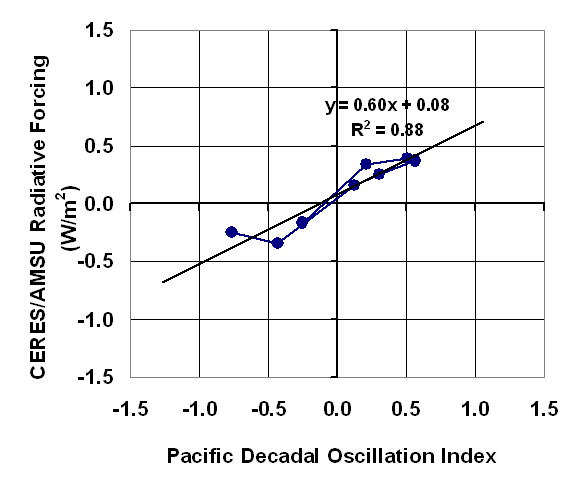
This internally-generated radiative forcing is most likely due to changes in global average cloud cover associated with the PDO. If we apply this relationship to yearly estimates of the PDO index, we get the following estimate of “internal radiative forcing” from the PDO since 1900:

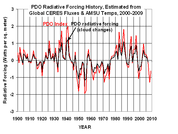
As can be seen, these radiative forcings – if they existed during the 20th Century– are comparable to the magnitude of the GISS forcings.

Model Simulations

The model has 7 free parameters that must be estimated to not only make a model run, but to then meaningfully compare that model run’s temperature “predictions” to the observed record of surface temperature variations. We are especially interested in what feedback parameter, when inserted in the model, best explains past temperature variations, since this determines the climate system’s sensitivity to increasing greenhouse gas concentrations.

Given some assumed history of radiative forcings like those shown above, these 7 model free parameters include:
1) An assumed feedback parameter
2) Total ocean depth that heat is stored/lost from.
3) Fraction of ocean depth contained in the upper ocean layer.
4) Ocean diffusion coefficient (same units as feedback parameter)
5) Initial temperature for 1st ocean layer
6) Initial temperature for 2nd ocean layer
7) Temperature offset for the observed temperature record

While the net feedback in the real climate system is likely dominated by changes in the atmosphere (clouds, water vapor, temperature profile), the model does not have an atmospheric layer per se. On the time scales we are considering here (1 to 5 years an longer), atmospheric temperature variations can be assumed to vary in virtual lock-step with the upper ocean temperature variations. So, the atmosphere can simply be considered to be a small (2 meter) part of the first ocean layer, which is the amount of water that has the same heat capacity as the entire atmosphere.

The last parameter, a temperature offset for the observed temperature record, is necessary because the model assumes some equilibrium temperature state of the climate system, a “preferred” temperature state that the model “tries” to relax to through the temperature feedback term in the model equations. This zero-point might be different from the zero-point chosen for display of observed global temperature anomalies, which the thermometer data analysts have chosen somewhat arbitrarily when compiling the HadCRUT3 dataset.

In order to sweep at least 10 values for every parameter, and run the model for all possible combinations of those parameters, there must be millions of computer simulations performed. Each simulation’s reconstructed history of temperatures can then be automatically compared to the observed temperature record to see how closely it matches.

So far, I have only run the model manually in an Excel spreadsheet, one run at a time, and have found what I believe to be the ranges over which the model free parameters provide the best match to global temperature variations since 1900. I expect that the following model fits to the observed temperature record will improve only slightly when we do full “Monte Carlo” set of millions of simulations.

All of the following simulation results use yearly running 5-year averages for the forcings for the period 1902 through 2007, with a model time step of 1 year.

CASE #1: All GISS Forcings
First let’s examine the best fit I found when I included all of the GISS forcings in the model runs. The following model best fit has a yearly RMS error of 0.0763 deg. C:

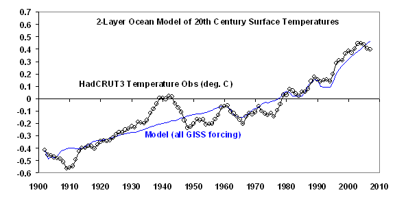
The above “best” model simulation preferred a total ocean depth of 550 meters, 10% of which (55 meters) was contained in the upper layer. (Note that since the Earth is 70% ocean, and land has negligible heat capacity, this corresponds to a real-Earth ocean depth of 550/0.7 = 786 meters).

The offset added to the HadCRUT3 temperature anomalies was very small, only -0.01 deg. C. The heat diffusion coefficient was 7 Watts per sq. meter per deg. C difference between the upper and lower ocean layers. The best initial temperatures of the first and second ocean layers at the start of the model integration were the same as the temperature observations for the first layer (0.41 deg. C below normal), and 0.48 deg. C below normal for the deeper layer.

What we are REALLY interested in, though, is the optimum net feedback parameter for the model run. In this case, it was 1.25 Watts per sq. meter per deg. C. This corresponds to about 3 deg. C of warming for a doubling of atmospheric carbon dioxide (2XCO2, based upon an assumed radiative forcing of 3.7 Watts per sq. meter for 2XCO2). This is in approximate agreement with the IPCC’s best estimate for warming from 2XCO2, and supports the realism of the simple forcing-feedback model for determining climate sensitivity.

But note that the above simulation has 2 shortcomings: 1) it does not do a very good job of mimicking the warming up to 1940 and subsequent slight cooling to the 1970s; and (2) other than the major volcanic eruptions (e.g. Pinatubo in 1991), it does not mimic the sub-decadal temperature variations.

CASE #2: All GISS Forcings except Tropospheric Aerosols
Since the tropospheric aerosols have the largest uncertainty, it is instructive to see what the previous simulation would look like if we remove all 3 tropospheric aerosol components (aerosol reflection, black carbon, and aerosol indirect effect on clouds).

In that case an extremely similar fit to Case #1 is obtained, which has only a slightly degraded RMS error of 0.0788 deg. C.

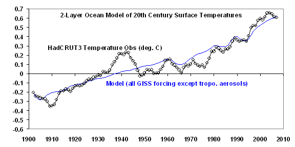
This reveals that the addition of the tropospheric aerosols in the first run improved the model fit by only 3.2% compared to the run without tropospheric aerosols. Yet, what is particularly important is that the best fit feedback has now increased from 1.25 to 3.5 Watts per sq. meter per deg. C, which then reduces the 2XCO2 climate sensitivity from 3.0 deg. C to about 1.1 deg. C! This is below the 1.5 deg. C lower limit the IPCC has ‘very confidently” placed on that warming.

This illustrates the importance of assumed tropospheric aerosol pollution to the IPCC’s global warming arguments. Since the warming during the 20th Century was not as strong as would some expected from increasing greenhouse gases, an offsetting source of cooling had to be found – which, of course, was also manmade.

But even with those aerosols, the model fit to the observations was not very good. That’s where the PDO comes in.

CASE #3: PDO plus all GISS Forcings except Tropospheric Aerosols
For our third and final case, let’s see what happens when we replace the GISS tropospheric aerosol forcings – which are highly uncertain – with our satellite-inferred record of internal radiative forcing from the PDO.

The following plot shows that more of the previously unresolved temperature variability during the 20th Century is now captured; I have also included the “all GISS forcings” model fit for comparison:

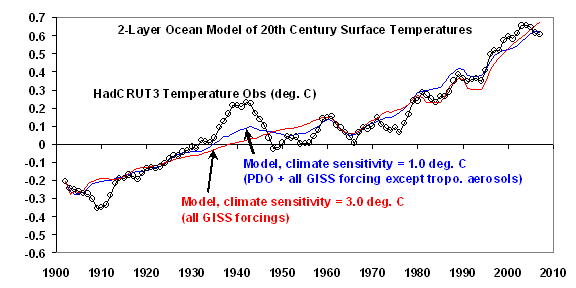
Using the satellite observed PDO forcing of 0.6 Watts per sq. meter per unit change in the PDO index, the RMS error of the model fit improves by 25.4%, to 0.0588 deg. C; this can be compared to the much smaller 3.2% improvement from adding the GISS tropospheric aerosols.

If we ask what PDO-related forcing the model “prefers” to get a best fit, the satellite-inferred value of 0.6 is bumped up to around 1 Watt per sq. meter per unit change in the PDO index, with an RMS fit improvement of over 30% (not shown).

In this last model simulation, note the smaller temperature fluctuations in the HadCRUT3 surface temperature record are now better captured during the 20th Century. This is evidence that the PDO causes its own radiative forcing of the climate system.

And of particular interest, the substitution of the PDO forcing for the tropospheric aerosols restores the low climate sensitivity, with a preferred feedback parameter of 3.6, which corresponds to a 2XCO2 climate sensitivity of only 1.0 deg. C.

If you are wondering, including BOTH the GISS tropospheric aerosols and the PDO forcing made it difficult to get the model to come close to the observed temperature record. The best fit for this combination of forcings will have to wait till the full set of Monte Carlo computer simulations are made.

Conclusions

It is clear (to me, at least) that the IPCC’s claim that the sensitivity of the climate is quite high is critically dependent upon (1) the inclusion of very uncertain aerosol cooling effects in the last half of the 20th Century, and (2) the neglect of any sources of internal radiative forcing on long time scales, such as the 30-60 year time scale of the PDO.

Since we now have satellite measurements that such natural forcings do indeed exist, it would be advisable for the IPCC to revisit the issue of climate sensitivity, taking into account these uncertainties.

It would be difficult for the IPCC to fault this model because of its simplicity. For global average temperature changes on these time scales, the surface temperature variations are controlled by (1) radiative forcings, (2) net feedbacks, and (3) heat diffusion to the deeper ocean. In addition, the simple model’s assumption of a preferred average temperature is exactly what the IPCC implicitly claims! After all, they are the ones who say climate change did not occur until humans started polluting. Think hockey stick.

Remember, in the big picture, a given amount of global warming can be explained with either (1) weak forcing of a sensitive climate system, or (2) strong forcing of an insensitive climate system. By ignoring natural sources of warming – which are understandably less well known than anthropogenic sources — the IPCC biases its conclusions toward high climate sensitivity. I have addressed only ONE potential natural source of radiative forcing — the PDO. Of course, there could be others as well. But the 3rd Case presented above is already getting pretty close to the observed temperature record, which has its own uncertainties anyway.

This source of uncertainty — and bias — regarding the role of past, natural climate variations to the magnitude of future anthropogenic global warming (arghh! I mean climate change) is something that most climate scientists (let alone policymakers) do not yet understand.