Guest post by John Christy, UAHuntsville, Alabama State Climatologist
(NOTE: Fig. 2.2 has now been extended in time.)
I was finishing up my U.S. Senate testimony for 1 Aug when a reporter sent me a PNAS paper by Hansen et al. (2012) embargoed until after the Hearing. Because of the embargo, I couldn�t comment about Hansen et al. at the Hearing. This paper claimed, among other things, that the proportion of the Northern Hemisphere land area (with weather stations) that exceeded extreme summer hot temperatures was now 10 percent or more for the 2006 to 2011 period.
For extremes at that level (three standard deviations or 3-sigma) this was remarkable evidence for �human-made global warming.� Statistically speaking, the area covered by that extreme in any given hotter-than-average year should only be in the lowest single digits � that is, if the Hansen et al. assumptions are true � i.e., (a) if TMean accurately represents only the effect of extra greenhouse gases, (b) if the climate acts like a bell-shaped curve, (c) if the bell-shaped curve determined by a single 30-year period (1951-1980) represents all of natural climate variability, and (d) if the GISS interpolated and extrapolated dataset preserves accurate anomaly values. (I hope you are raising a suspicious eyebrow by now.)
The conclusion, to which the authors jumped, was that such a relatively large area of recent extremes could only be caused by the enhanced greenhouse effect. But, the authors went further by making an attempt at advocacy, not science, as they say they were motivated by �the need for the public to appreciate the significance of human-made global warming.�
Permit me to digress into an opinionated comment. In 2006, President George W. Bush was wrong when he said we were addicted to oil. The real truth is, oil, and other carbon-based fuels, are merely the affordable means by which we can satisfy our true addictions � long life, good health, prosperity, technological progress, adequate food supplies, internet services, freedom of movement, protection from environmental threats, and so on. As I�ve said numerous times after living in Africa, – without energy, life is brutal and short.
Folks with Hansen�s view are quick to condemn carbon fuels while overlooking the obvious reasons for their use and the astounding benefits they provide (and in which they participate). The lead author referred to coal trains as �death trains – no less gruesome than if they were boxcars headed to the crematoria.� The truth, in my opinion, is the exact opposite � carbon has provided accessible energy that has been indisputably responsible for enhancing security, longevity, and the overall welfare of human life. In other words, carbon-based energy has lifted billions out of an impoverished, brutal existence.
In my view, that is �good,� and I hope Hansen and co-authors would agree. I can�t scientifically demonstrate that improving the human condition is �good� because that is a value judgment about human life. This �good� is simply something I believe to be of inestimable value, and which at this point in history is made possible by carbon.
Back to science. After reading Part 1, everyone should have some serious concerns about the methodology of the Hansen et al. as published in PNAS. [By the way, I went through the same peer-review process for this post as for a PNAS publication: I selected my colleague Roy Spencer, a highly qualified, award-winning climate scientist, as the reviewer.]
With regard to (a) above, I�ve already provided evidence in Part 1 that TMean misrepresents the response of the climate system to extra greenhouse gases. So, I decided to look only at TMax. For this I downloaded the station data from the Berkeley BEST dataset (quality-controlled version). This dataset has more stations than GISS, and can be gridded so as to avoid extrapolated and interpolated values where strange statistical features can arise. This gridding addresses assumption (d) above. I binned the data into 1� Lat x 2� Lon grids, and de-biased the individual station time series relative to one another within each grid, merging them into a single time series per grid. The results below are for NH summer only, to match the results that Hansen et al. used to formulate their main assertions.
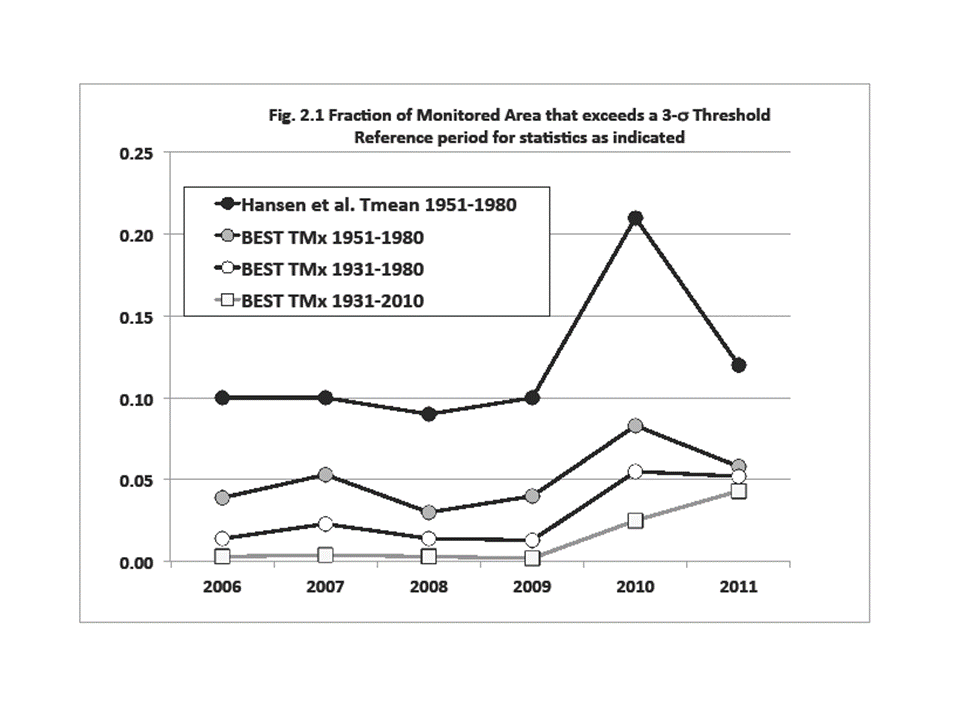
In Fig. 2.1 I show the percentage of the NH land areas that Hansen et al. calculated to be above the TMean 3-sigma threshold for 2006 to 2011 (black-filled circles). The next curve (gray-filled circles) is the same calculation, using the same base period (1951-1980), but using TMax from my construction from the BEST station data. The correlation between the two is high, so broad spatial and temporal features are the same. However, the areal coverage drops off by over half, from Hansen�s 6-year average of 12 percent to this analysis at 5 percent (click for full-size version):
Now, I believe assumption (c), that the particular climate of 1951-1980 can provide the complete and ideal distribution for calculating the impact of greenhouse gas increases, displays a remarkably biased view of the statistics of a non-linear dynamical system. Hansen et al. claim this short period faithfully represents the natural climate variability of not just the present, but the past 10,000 years – and that 1981-2011 is outside of that range. Hansen assuming any 30-year period represents all of Holocene climate is simply astounding to me.
A quick look at the time series of the US record of high TMax�s (Fig.1.1 in Part 1) indicates that the period 1951-1980 was one of especially low variability in the relatively brief 110-year climate record. Thus, it is an unrepresentative sample of the climate�s natural variability. So, for a major portion of the observed NH land area, the selection of 1951-80 as the reference-base immediately convicts the anomalies for those decades outside of that period as criminal outliers.
This brings up an important question. How many decades of accurate climate observations are required to establish a climatology from which departures from that climatology may be declared as outside the realm of natural variability? Since the climate is a non-linear, dynamical system, the answer is unknown, but certainly the ideal base-period would be much longer than 30 years thanks to the natural variability of the background climate on all time scales.
We can test the choice of 1951-1980 as capable of defining an accurate pre-greenhouse warming climatology. I shall simply add 20 years to the beginning of the reference period. Certainly Hansen et al. would consider 1931-1950 as �pre-greenhouse� since they considered their own later reference period of 1951-1980 as such. Will this change the outcome?
The result is the third curve from the top (open circles) in Fig. 2.1 above, showing values mostly in the low single digits (6-year average of 2.9 percent) being generally a quarter of Hansen et al.�s results. In other words, the results change quite a bit simply by widening the window back into a period with even less greenhouse forcing for an acceptable base-climate. (Please note that the only grids used to calculate the percentage of area were those with at least 90 percent of the data during the reference period � I couldn�t tell from Hansen et al. whether they had applied such a consistency test.)
The lowest curve in Fig. 2.1 (squares) uses a base reference period of 80 years (1931-2010) in which a lot of variability occurred. The recent decade doesn�t show much at all with a 1.3 percent average. Now, one may legitimately complain that since I included the most recent 30 years of greenhouse warming in the statistics, that the reference period is not pure enough for testing the effect. I understand fully. My response is, can anyone prove that decades with even higher temperatures and variations have not occurred in the last 1,000 or even 10,000 pre-greenhouse, post-glacial years?
That question takes us back to our nemesis. What is an accurate expression of the statistics of the interglacial, non-greenhouse-enhanced climate? Or, what is the extent of anomalies that Mother Nature can achieve on her own for the �natural� climate system from one 30-year period to the next? I�ll bet the variations are much greater than depicted by 1951-1980 alone, so this choice by Hansen as the base climate is not broad enough. In the least, there should be no objection to using 1931-1980 as a reference-base for a non-enhanced-greenhouse climate.
In press reports for this paper (e.g., here), Hansen indicated that �he had underestimated how bad things could get� regarding his 1988 predictions of future climate. According to the global temperature chart below (Fig. 2.2), one could make the case that his comment apparently means he hadn�t anticipated how bad his 1988 predictions would be when compared with satellite observations from UAH and RSS:
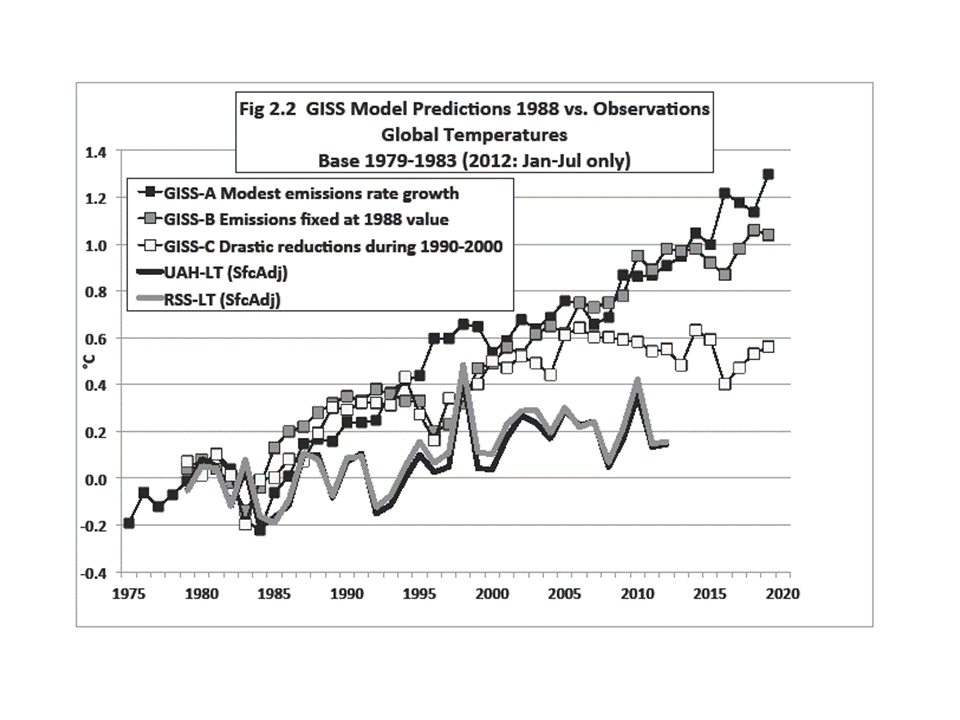
By the way, a climate model simulation is a hypothesis and Fig. 2.2 is called �testing a hypothesis.� The simulations fail the test. (Note that though allowing for growing emissions in scenario A, the real world emitted even more greenhouse gases, so the results here are an underestimate of the actual model errors.)
The bottom line of this little exercise is that I believe the analysis of Hansen et al. is based on assumptions designed to confirm a specific bias about climate change and then, like a legal brief, advocates for public acceptance of that bias to motivate the adoption of certain policies (see Hansen�s Washington Post Op-Ed 3 Aug 2012).
Using the different assumptions above, which I believe are more scientifically defensible, I don�t see alarming changes. Further, the discussion in and around Hansen et al. of the danger of carbon-based energy is simply an advocacy-based opinion of an immensely complex issue and which ignores the ubiquitous and undeniable benefits that carbon-based energy provides for human life.
Finally, I thought I just saw the proverbial �horse� I presumed was dead twitch a little (see Part 1). So, I want to beat it one more time. In Fig. 2.3 is the 1900-2011 analysis of areal coverage of positive anomalies (2.05-sigma or 2.5 percent significance level) over USA48 from the BEST TMax and TMin gridded data. The reference period is 1951-1980:
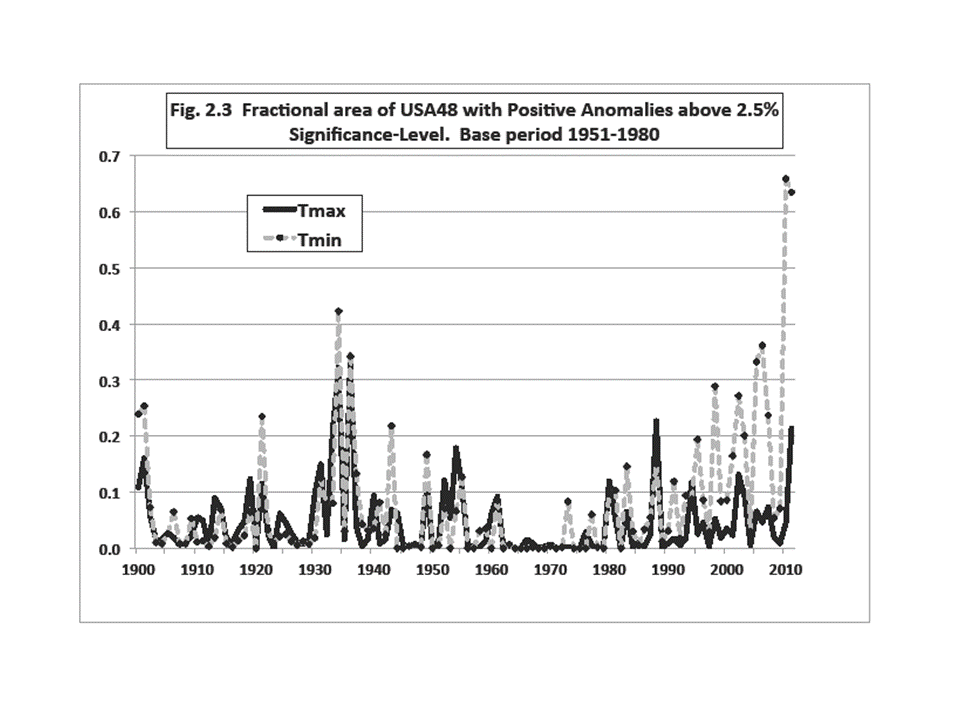
Does anyone still think TMax and TMin (and thus TMean) have consistently measured the same physical property of the climate through the years?
It�s August and the dewpoint just dipped below 70�F here in Alabama, so I�m headed out for a run.
REFERENCE:
Hansen, J., M. Sato and R. Ruedy, 2012: Perception of climate change. Proc. Nat. Ac. Sci., doi/10.1073/pnas.1205276109.

 Home/Blog





Cela a un impression ngatif pour les entreprises
en cas de dprciation des cryptomonnaies,
puisque ces baisses ne sont pas enregistres
comme des pertes du point de vue comptable.
The information on this article is so wonderful, thanks for sharing this! Good job!
https://emergencyplumberbondi.net.au/emergency-plumber-bondi/
Heya i’m for the first time here. I came across this board and I find It really useful & it helped
me out much. I hope to present one thing again and aid others like you helped me.