
 Home/Blog
Time lapse video of Spica and Comet ISON rising, Nov. 20, 2013, over northeast Alabama. It was very windy, so there is a little camera shake as it zooms in from full frame to 130% crop. Composed of 326 frames from a Canon 6D, Canon 200mm f/2.8 lens (@ f/5.6), ISO 1600, 30 sec exposures. Tracking with AstroTrac. Note the movement of the comet past the neighboring stars late in the video.
Archive for 2013
Spica & Comet ISON Rising, Nov. 20, 2013
Wednesday, November 20th, 2013Comet ISON & Moonlit Clouds, I & II (time lapse)
Monday, November 18th, 2013I took these this morning (Nov. 18, 2013), again near New Market, Alabama. I was hoping the clouds would clear in time to reveal the comet, which is just what happened. The first video is from ~300 20-sec exposures, the 2nd video used ~150 5-sec exposures (shot just after the first). I used a Canon 6D with 85mm f/1.2 lens and an AstroTrac for tracking of the stars. All of the lighting of the landscape was provided by the moon and the very sensitive camera and lens…by eye, it was much darker.
Comet ISON Rising, 14 Nov. 2013
Thursday, November 14th, 2013UPDATE (11/16/2013): I’ve replaced the video with one that pans and zooms…much better. (The video will keep looping after it loads):
This is my latest (and best) attempt at a time lapse video of Comet ISON, rising over a heavily forested area of northeast Alabama.
The video starts without tracking, so the stars are streaked. Then I turned on star tracking when the comet was approximately centered in the frame, and the frame of reference “launches” to keep up with the comet.
I was finally able to see the comet for the first time in my Canon 10×30 binoculars….I could barely make out the faint tail. But you need dark skies and know just where to look. To find it, I’m now using the iPhone app “Star Walk“, which is absolutely amazing.
This time I used my new Canon 85mm f/1.2 lens, stopped down to f/2.5, 30 sec exposures. This very fast lens is awesome…it seems to show more detail than my 200mm lens extended to 400mm with a 2x extender. The video is cropped to 120% of full pixel resolution, so the effective magnification is about 6x or 7x.
There is an interesting satellite which passes to the left of the comet, from top to bottom. It crosses the sky much slower than most satellites, suggesting a very high orbital altitude. Based upon the direction and the angular speed (the 30 sec satellite streaks are same length as the star streaks at the beginning of the video), it appears to be geostationary (wow! Imaging a geostationary satellite with a 85 mm lens!).
PLUS…if you look closely, in one frame a meteor streaks by the geostationary satellite!
UPDATE: It appears the geostationary satellite passing by ISON was either Intelsat 905 or 907, which passed by (as seen from from my location) close to 4:30 a.m. These satellites are near the Equator off the coast of Africa, around 25W longitude, at an altitude of ~22,000 miles.
UPDATE #2: The bright satellite that whizzed by ISON just before the geostationary satellite appears to be an Atlas 5 Centaur booster rocket from a March 10, 2007 DoD NEXTSat launch.
Typhoon Haiyan: My debate on CNN Piers Morgan Live last night
Tuesday, November 12th, 2013I reaallly didn’t want to do this. I was deliriously tired from getting up at 2 a.m. every morning to chase Comet ISON, and I knew it would probably be a hostile environment on Piers Morgan Live.
Piers himself was polite, but the guy they had covering the opposite view on the recent typhoon in the Philippines, “environmental correspondent” Mark Hertsgaard of The Nation, pulled out all the stops. Using the D-word, accusing me of scientific malpractice, etc. It was hard to get a word in edgewise.
Oh well, I’ll let the video speak for itself. If nothing else, it’s fairly entertaining. [They cut out the first part of the interview, where I explain that Typhoon Haiyan was not the biggest typhoon on record…maybe someone can find the full version of this interview for us.]
UAH v5.6 Global Temperature Update for October, 2013: +0.29 deg. C
Tuesday, November 12th, 2013We finally received the missing NOAA-19 and Metop2 AMSU data from NESDIS, resulting from the government shutdown, covering the first half of October. For some reason we got all of the NOAA-15 and NOAA-18 data, but the other two satellite feeds were stopped.
So, the numbers below supersede the UAH October temperature press release, which was sent out by accident. (The global anomaly map for October was approximately correct, though, because it was based upon the 2 satellites which had complete data coverage for the month).
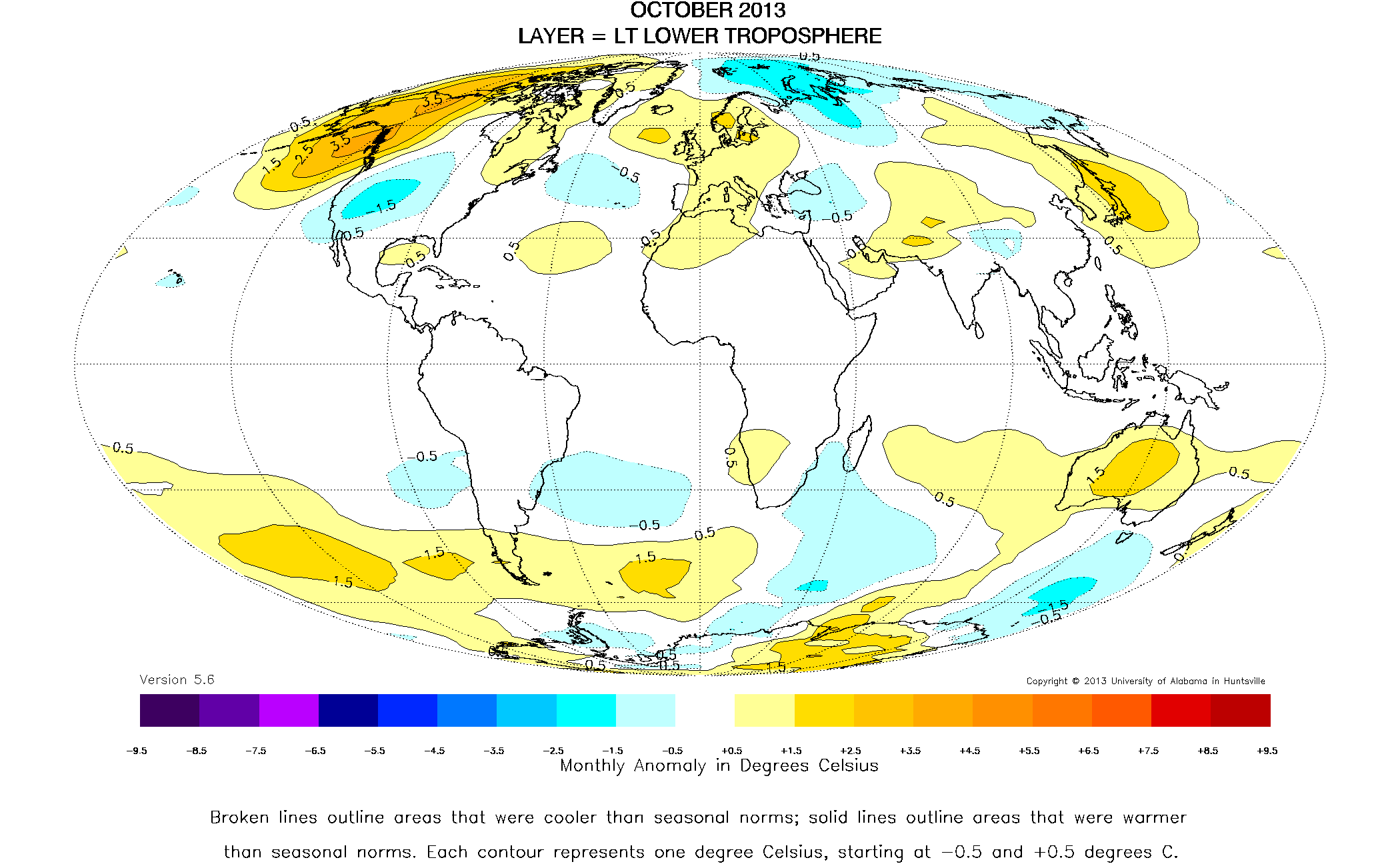
The Version 5.6 global average lower tropospheric temperature (LT) anomaly for October, 2013 is +0.29 deg. C (click for larger version):
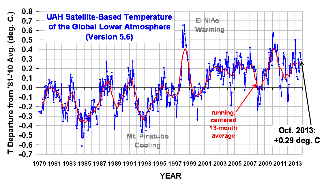
The global, hemispheric, and tropical LT anomalies from the 30-year (1981-2010) average for the last 10 months are:
YR MON GLOBAL NH SH TROPICS
2013 01 +0.496 +0.512 +0.481 +0.387
2013 02 +0.203 +0.372 +0.033 +0.195
2013 03 +0.200 +0.333 +0.067 +0.243
2013 04 +0.114 +0.128 +0.101 +0.165
2013 05 +0.082 +0.180 -0.015 +0.112
2013 06 +0.295 +0.335 +0.255 +0.220
2013 07 +0.173 +0.134 +0.211 +0.074
2013 08 +0.158 +0.111 +0.206 +0.009
2013 09 +0.365 +0.339 +0.390 +0.189
2013 10 +0.290 +0.329 +0.250 +0.032
Popular monthly data files:
uahncdc_lt_5.6.txt (Lower Troposphere)
uahncdc_mt_5.6.txt (Mid-Troposphere)
uahncdc_ls_5.6.txt (Lower Stratosphere)
Our new paper: El Nino warming reduces climate sensitivity to 1.3 deg. C
Monday, November 11th, 2013
Al Gore meets his match.
Our new paper has finally appeared in Asia Pacific Journal of Atmospheric Science (APJAS). Entitled “The Role of ENSO in Global Ocean Temperature Changes during 1955-2011 Simulated with a 1D Climate Model“, we use a time-dependent forcing-feedback model of global average ocean temperature as a function of depth to explain the Levitus record ocean temperature variations and trends since 1955.
The modeling philosophy is to answer the question: What combination of net feedback (climate sensitivity) and ocean mixing best explain the observed global average ocean temperature variations since 1955? In the global average, temperature variations are the result of only 3 processes: Forcing, feedback, and ocean mixing. These can be addressed in a simple 1D model.
Our primary interest was to explore how El Nino and La Nina activity since the 1950s affect our interpretation of climate sensitivity. Basically, if all of the ocean warming in the last 50 years (assuming it is real and accurate) has been due to anthropogenic greenhouse gas emissions, it leads to a higher climate sensitivity. But if some of that warming was due to stronger El Nino activity (since the 1970s) it would lead to a lower climate sensitivity. We let a variety of observations tell us how the various influences combine to cause climate change, by varying the model “free” parameters over many thousands of combinations to find a best match to the observations.
We examine three scenarios, shown schematically below.
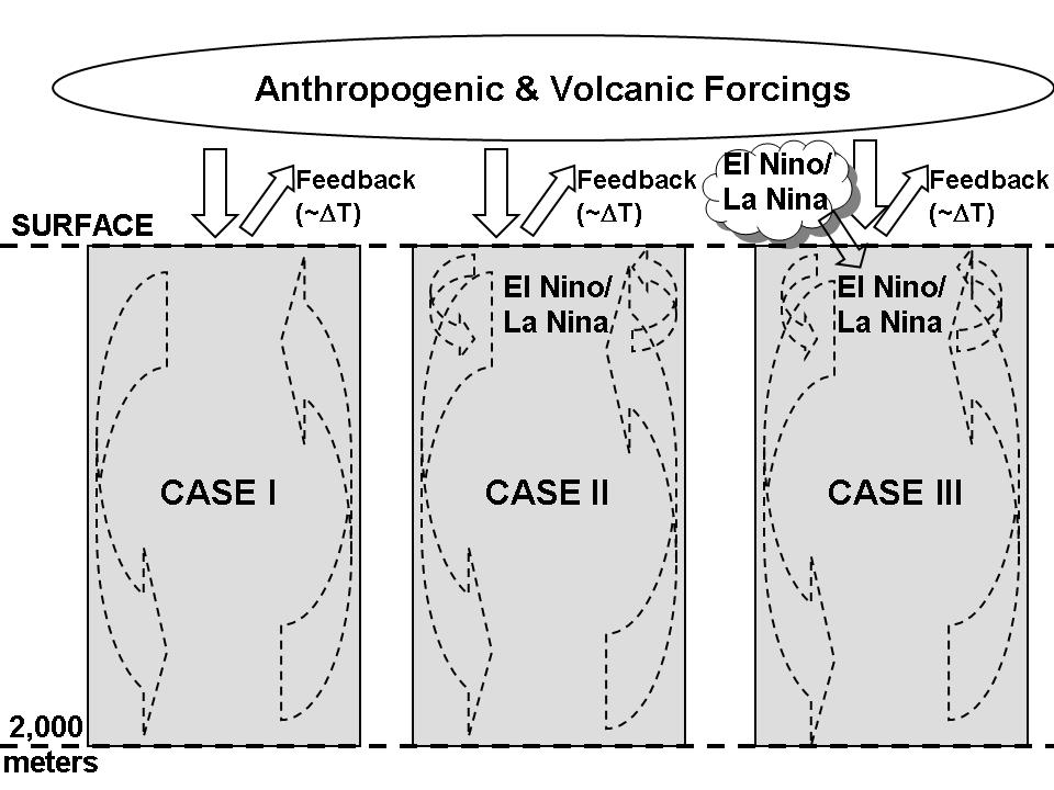
Schematic representation of the 1D forcing-feedback-mixing model. Solid arrows represent radiative energy exchanges, while dashed arrows represent non-radiative energy exchanges.
The first case (CASE I) uses only the RCP radiative forcings (also used by the latest crop of IPCC climate models) to see if we get about the same climate sensitivity as those models get (under the VERY important assumption that those are the ONLY forcings causing warming since the 1950s). This is sort of a sanity check on the model. We run the model with thousands of combinations of climate sensitivity and ocean mixing to get an approximate best-match with the Levitus observations.
In that case we get about 2.2 deg. C of equilibrium warming in response to a doubling of atmospheric CO2, somewhat below the average of the IPCC models. The model fits to the ocean temperature trends as a function of depth are shown in the next figure:
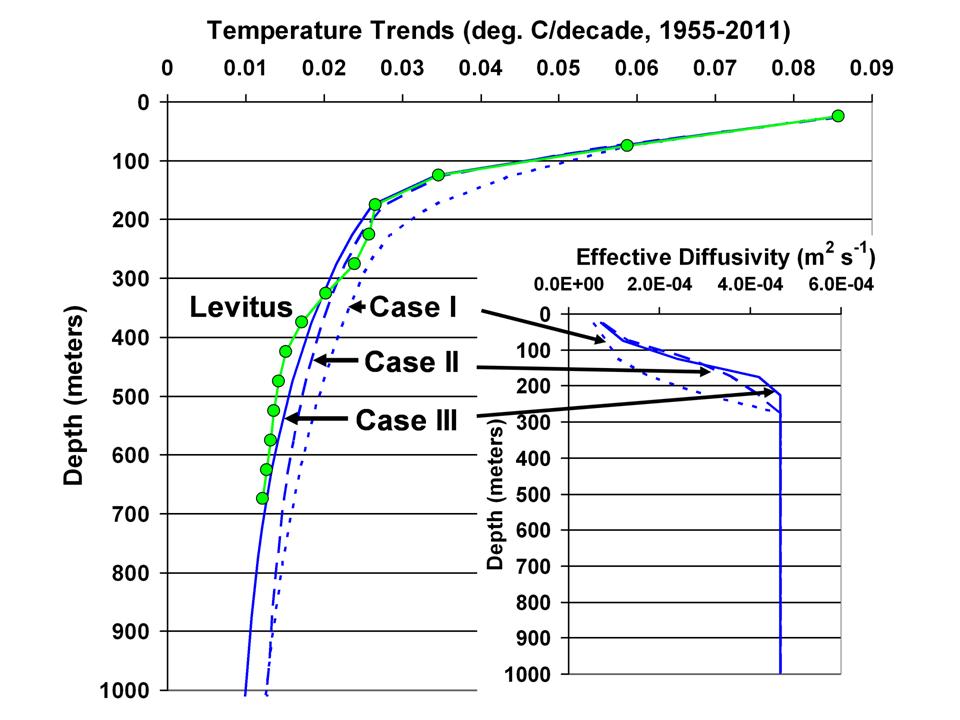
Comparison of three model cases to observed decadal ocean temperature trends as a function of depth, in 50 m layers, for 1955-2011. The layer effective diffusivities used in the model simulations are shown in the inset.
In the second case (CASE II), we add the observed history of El Nino and La Nina activity (from the Multivariate ENSO Index, or MEI) as a change in ocean mixing alone. Basically, using the ocean temperature vs. MEI variations as a guide, we warm the top 100 m of ocean and cool the 100-200 m layer by exactly offsetting amounts, thus conserving thermal energy, in proportion to the strength of El Nino activity. The opposite is done for La Nina activity. Case II leads to a slightly lower climate sensitivity, 2.0 deg. C.
But the third case (CASE III) is the one we were really interested in, because it addresses the debate we have with Andy Dessler over the role of cloud variations associated with El Nino and La Nina. I maintain that the global atmospheric circulations associated with El Nino lead to a slight reduction in global albedo, and so a portion of El Nino warming is actually due to radiative warming of the system, not just a temporary reduction in upwelling of colder water.
In other words, in addition to the model specified feedback parameter (climate sensitivity) which determines how much radiative energy is lost by the Earth to space in response to warming, we also allow the model to change the Earth’s radiative balance preceding warming (or cooling) due to El Nino (or La Nina). The time lead or lag of this “internal radiative forcing” is adjustable, and the model “decides” the best match to the observations.
The observations we use to help guide the model fit is the CERES-observed changes in the global oceanic radiative budget since March 2000. The lag regression plot of these changes in Earth’s radiative budget versus HadSST2 sea surface temperatures shows that only when we include the “internal radiative forcing” aspect of ENSO does the model behavior show the lead-lag behavior seen in the satellite observations:
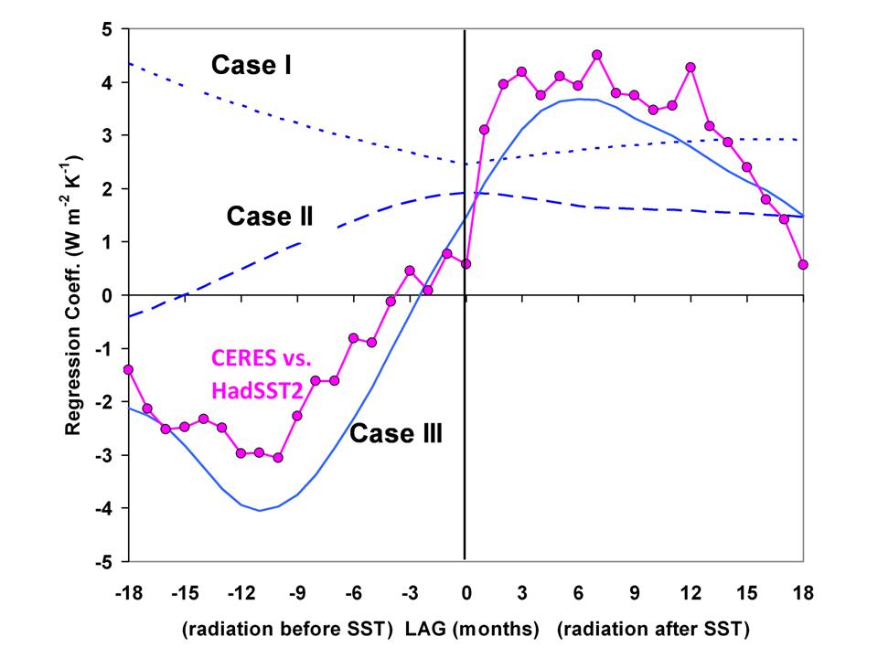
Lag regression coefficients between monthly CERES radiative fluxes and HadSST2 sea surface temperature variations, and compared to the three model simulations
Significantly, when the natural radiative warming effect of El Nino is included, the climate sensitivity is reduced substantially — to 1.3 deg. C.
Basically, a portion of El Nino warming is radiatively forced, probably due to a decrease in low clouds allowing more sunlight in, with the model choosing a 9 month average time lag of the cloud changes preceding the ENSO activity changes.
So, when the Earth went through a ~30 year period of more intense El Nino activity after the mid 1970s, a portion of the warming we experienced was caused by the more frequent El Nino activity. (Although not in the paper, we also found that the model explains the warming before 1940 as a response to stronger El Nino activity back then, as well as the slight cooling from the 1940s to the 1970s from stronger La Nina activity).
Here’s the model response by year for the three Cases, for the 0-50m layer ocean temperature (note how stronger La Ninas explain the lack of recent warming, Case III vs. Case I):
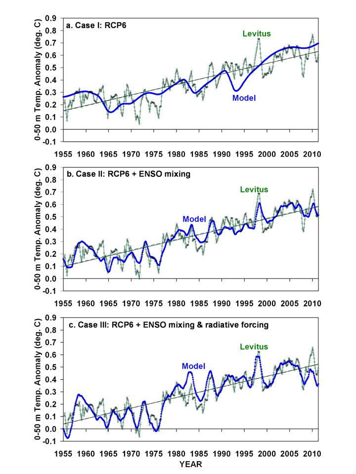
Model simulations of monthly global average 0-50 m layer ocean temperature variations for three cases: (a) only RCP6 radiative forcings; (b) RCP6 plus ENSO-related non-radiative forcing (ocean mixing); and (c) RCP6 plus ENSO-related radiative and non-radiative forcings.
This ENSO-climate change connection has, of course, been hypothesized by others. What we have done is to provide a stronger physically-based framework for quantifying that connection. For example, we find that 1 unit of MEI index (which is 1 standard deviation in the El Nino direction) causes a 0.6 W/m2 of radiative forcing of the climate system.
Again, the model only reproduces the CERES satellite-observed behavior when the radiative budget changes precede the El Nino and La Nina activity, suggesting a cause-and-effect connection. And when that is included, the optimum climate sensitivity chosen by the model is considerably below what the IPCC claims is reasonable for expected warming in our future.
Some of you might recall that Andy Dessler tried to get me to admit that my position was equivalent to saying that “clouds cause El Nino”, which would be inaccurate. What I am saying is that El Nino is associated with changes in Earth’s radiative balance which are not just a feedback response to surface warming, but also force some of that warming. When that “internal radiative forcing” effect is included, optimizing the agreement with 10 years of satellite radiative budget measurements, it considerably reduces the diagnosed sensitivity of the climate system.
In simple terms, the climate system is chaotic, capable of causing global warming (or cooling) all by itself. There probably is no magical normal average albedo, keeping the same amount of sunlight coming in to the climate system year after year. As I keep reminding people, the increase in ocean heat content over the last 50 years is equivalent to a 1 part in 1,000 change in average radiative energy flows. Do we really think nature cannot cause such small changes all by itself?
There needs to be more studies of this type, and I am at a loss to explain why they haven’t been performed. They are relatively easy, and don’t require a marching army of climate modelers. Yet, I will tell you that it is virtually impossible for someone like me to get a proposal specifically funded to perform such a study, because a few gatekeepers in the science community make sure during the peer review process that it doesn’t happen. Instead, we have to piggy-back on other funded projects we have.
I would hope that a simple model like the one we used can help guide the development of the more sophisticated, 3D models. Find a simple, physically-based model that best matches a variety of observations, and add complexity to the model only when it is required to explain observations which the simple model cannot explain.
That’s the way much of science is traditionally done…why not climate science?
Maybe simple modeling studies will gradually emerge from the mainstream climate community, especially with the glaring 15+ year hiatus in warming which is currently being swept under the rug. When they do, I predict it will end up being “their” discovery, not the few skeptics who are working this issue. But I’ve been down this road before, in a previous research life, and I’m OK with that.
Finally, this study leaves open the question of what other natural warming mechanisms there might be out there. We have only addressed ENSO, which alone reduced the diagnosed climate sensitivity in response to increasing CO2 to only 1.3 deg. C, a level I would consider benign or even beneficial. We say nothing about what else might be contributing to warming — I suspect we have already rocked the boat too much.
Comet ISON time lapse, Nov. 11, 2013
Monday, November 11th, 2013This is my third attempt at a time lapse video of Comet ISON from this morning, Nov. 11, 2013, near New Market, Alabama.
I used a Canon 6D with Canon 200mm f/2.8 lens with Canon 2x extender, at f/16, ISO 1600, 77 60-sec exposures. Tracking with Astrotrac on a Ravelli tripod. Temperature was about 43 deg F.
Comet ISON time lapse video, Take 2
Friday, November 8th, 2013My second attempt at a time lapse video of Comet ISON, this time from a dark sky location on a mountaintop near New Market, Alabama, morning of Nov. 8, 2013.
I’m learning how frustrating astrophotography with a telephoto lens can be. This time I learned the hard way: double-check the focus!! Focusing on stars with a telephoto lens is difficult, especially when working at 400 mm focal length. This video would have been so much better with crisp focus, I could have zoomed in considerably through cropping.
I will try again in a few days, weather permitting, before the pre-dawn sky gets too bright. Maybe ISON will also brighten in the meantime. (After the video loads, it should loop by itself):
Storminess and the Inefficient Atmospheric Heat Engine
Wednesday, November 6th, 2013There is an aspect of weather generation and storminess that I never see discussed, and which I think could be important to understand when discussing possible changes in weather with climate change.
It has long been known that the atmosphere is a very inefficient heat engine. The rate of kinetic energy generation supporting the atmospheric circulation is only about 1% of the rate of solar heating (e.g. Peixoto J P and Oort A H 1992 Physics of Climate). Since most of what we perceive as weather is related to wind, one way or another, we can roughly say that only 1% of the solar energy absorbed by the Earth goes into the creation of weather systems.
I suspect that when we see periods of greater or lesser storminess on a global basis, we are seeing fluctuations in this efficiency. If air mass temperature differences build up over a period of days or weeks, say with cold winter air masses over N. America or Asia intensifying in the winter, the temperature contrast (available energy) for the creation of storms increases. (I would imagine that storminess was considerably more energetic during the ice age(s)…I’m sure someone has researched this issue before.)
Since it takes time for low pressure systems to form and draw upon this potential energy from the temperature contrast between air masses, there is a time lag involved in the cycles of storminess. The potential energy built up is released as low pressure areas form and their circulations cause warm air to rise up and flow over the cold air masses, and the cold air slides under and displaces the warm air masses.
Global warming theory has traditionally expected that the equator-to-pole gradient in temperature would be reduced during warming. Observations suggest this has indeed occurred, at least over the Northern Hemisphere. So, the energy available for storm formation has decreased. I suspect the effect is small, though. (Storminess is also related to the tropospheric vertical temperature lapse rate…a steeper lapse rate can support more kinetic energy generation).
[By the way, I don’t think the decrease in the equator-to-pole temperature contrast is a fingerprint of human-induced warming…it’s a reflection of the geographic distribution of land, which will warm faster than the ocean no matter the cause of the warming.]
What is interesting about the 1% efficiency is how small that number is, which is related to the fact that weather is driven by relatively small temperature contrasts over relatively large distances: a few degrees over hundreds or thousands of kilometers. In a car engine, which can also be considered a heat engine with about 25% efficiency, the mechanical work that is done is drawing on temperature differences of hundreds of degrees over a few inches.
If the atmospheric heat engine efficiency were to increase from an average of 1% to 2%, that would be a doubling of the kinetic energy involved in weather systems…yet the thermodynamic efficiency would still be very low.
What does all of this have to do with global warming? I don’t know…I just think it’s interesting.
Comet ISON time lapse – my first attempt
Saturday, November 2nd, 2013I’ve been curious whether I could pull off a time lapse video of Comet ISON using relatively modest camera equipment and a telephoto lens. Professional photographer Justin Ng used a 20 inch (!) telescope and a monochrome CCD camera to do the same thing several days ago. I told him about attempting it with a 400 mm lens and camera and he was (justifiably) skeptical, but wished me luck.
My first attempt was this morning, and the results seem good enough to try again in a couple days at a dark sky location. Despite moderate city light pollution and some clouds, I captured the green glow of Comet ISON in 52 frames (try the “full screen” icon):
Comet ISON time lapse – first attempt from Roy Spencer on Vimeo.
I had difficulty finding the comet at first…I forgot my binoculars and had to guess where it was based upon online tracking maps…it’s currently near the back “foot” of Leo. I doubt I would have seen it in the binoculars anyway because it is still so faint.
I’m also using an AstroTrac for the first time, which allows you to track the stars with a camera tripod. My polar alignment wasn’t the best, so the stars are still moving across the camera’s field of view, but it was good enough to keep the stars from trailing in the individual 60 sec exposures.
For reference, here’s Justin Ng’s time lapse using that humongous telescope and B&W CCD camera:
Journey of Comet ISON on 27 October 2013 from Justin Ng Photo on Vimeo.


