
 Home/Blog
Now that the CERES radiative flux products from the NASA Terra and Aqua satellites have been updated through October, 2013, I thought I would update the comparison between global average SST variations and CERES to examine forcing and feedback issues.
As in my recent post on SSM/I ocean variables, all plots below are for the global area-average ice-free ocean between 60 deg. North and South latitudes.
Starting with the SST variations, with the anomalies computed relative to the CERES period (March 2000 thru October 2013), we see that global average SST is reasonably well correlated with ENSO activity, which I am representing with the Multivariate ENSO Index (MEI). (Linear trend lines are for entertainment purposes only).
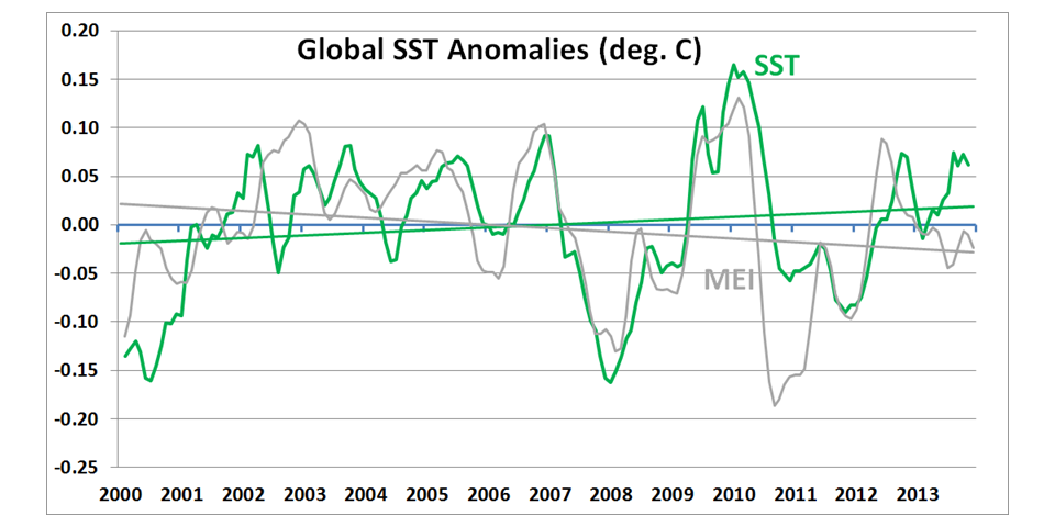
Fig. 1. Three-month anomalies in global average SST and MEI (scaled to SST) between March 2000 and October 2013.
The corresponding CERES radiative flux anomalies computed over the ocean also show a response to ENSO activity.
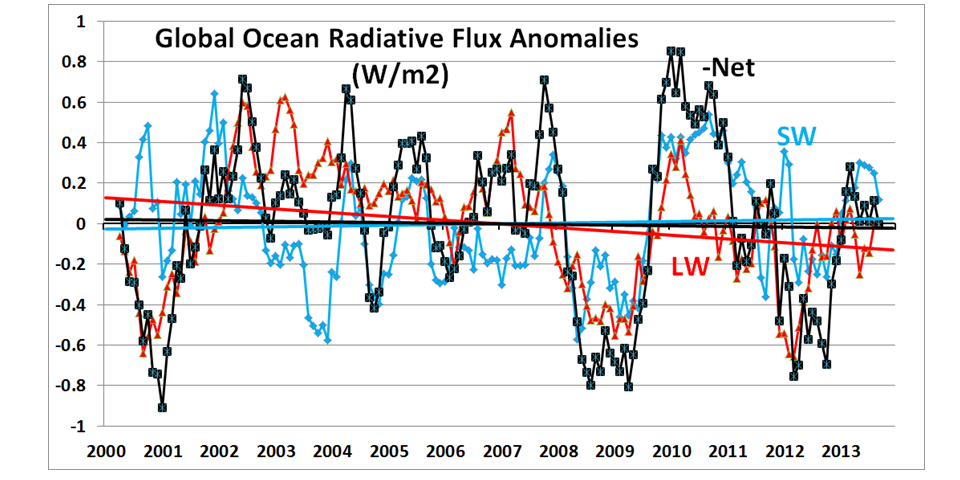
Fig. 2. Three-month global ocean anomalies in CERES all-sky radiative fluxes.
But in order to put the above pieces of the puzzle together, I have found that lag regression between SST and the other variables leads to considerable physical insight. The following plot shows how different variables change before and after SST during the 13+ year CERES period of record.
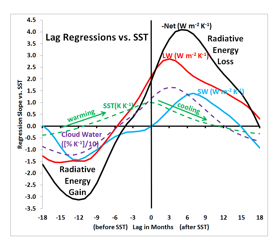
Fig. 3. Lag regression coefficients between SST and several other variables, based upon monthly running 3-month average global ocean anomalies.
We see that 12-18 months before peak SST is reached, there is a radiative accumulation of energy, both solar shortwave (SW) and infrared longwave (LW). (Net is close to the sum of the two, but with the sign flipped, so that positive numbers represent energy lost by the climate system).
The curve based upon SSM/I cloud water shows that there is a ~1% decrease in cloud water over the ocean about 9-18 months before peak SST anomalies of ~0.1 deg. C are reached, which probably explains the solar SW curve. This is the “internal radiative forcing” we talk about…the climate system’s cloud cover is not constant, and varies depending on circulation regime (El Nino or La Nina), creating a forcing of later temperature change.
As peak temperatures are approached (at zero time lag), the radiative fluxes change to a net loss, which continues for many months as SSTs then cool.
As long-time loyal readers of my blog are aware, the regression relationships at zero time lag are what are traditionally used to estimate feedbacks in the climate system, a methodology which I (and Lindzen) believe is seriously in error. Since feedbacks determine climate sensitivity, and sensitivity determines how much anthropogenic global warming there will be, this is a critical issue.
I�ve spent years studying this problem in considerable detail, and I don�t see any way yet to diagnose feedback (the radiative response to a temperature change) when there is a simultaneous, unknown, radiative forcing of temperature change going on.
The climate system is constantly out of balance, and without knowing how much internal radiative forcing is occurring, you can�t know the size of the net feedback. Radiative forcing always opposes net radiative feedback, and if forcing is occurring, any estimate of feedback is biased in the direction of positive feedback (high climate sensitivity).
We have three papers published on this (Lindzen has others), and as far as I can tell, the climate community still does not understand the implications of our work.
What we do know is that the climate models we have analyzed show relationships that depart significantly from the observations, and in the direction of high climate sensitivity. Our most significant papers on this, which I fully stand behind, are here and here. (The latter paper is the one that led to the journal editor resigning and apologizing to Trenberth for allowing to be published…even though it was peer reviewed, and never retracted.)
This is a subject on which the scientific consensus, as far as I can tell, is clueless. Attempts to refute our work have been feeble at best. Andy Dessler claims the radiative signals are all feedback (no “internal forcing”) and are a response to previous temperature changes.
Well, if that is the case (as I have asked him), why doesn’t he then use a time lag in his feedback diagnoses? As Lindzen has shown, when this is done you diagnose strong negative feedback. Oops…wrong answer for the IPCC.
To paraphrase Trenberth, we can’t account for the IPCC�s continuing to ignore this issue, and it is a travesty that we can’t. 😉
For those interested in the data which went into the above plots, here is the spreadsheet.


