What can we learn from the IPCC climate models based upon their ability to reconstruct the global average surface temperature variations during the 20th Century?

While the title of this article suggests I’ve found evidence of natural climate cycles in the IPCC models, it’s actually the temperature variability the models CANNOT explain that ends up being related to known climate cycles. After an empirical adjustment for that unexplained temperature variability, it is shown that the models are producing too much global warming since 1970, the period of most rapid growth in atmospheric carbon dioxide. This suggests that the models are too sensitive, in which case they are forecasting too much future warming, too.

Climate Models’ 20th Century Runs
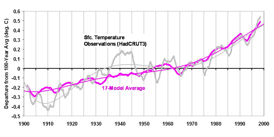
We begin with the IPCC’s best estimate of observed global average surface temperature variations over the 20th Century, from the “HadCRUT3” dataset. (Monthly running 3-year averages are shown throughout.) Of course, there are some serious concerns over the validity of this observed temperature record, especially over the strength of the long-term warming trend, but for the time being let’s assume it is correct (click on image to see a large version).

Also shown in the above graph is the climate model temperature reconstruction for the 20th Century averaged across 17 of the 21 climate models which the IPCC tracks. To provide a reconstruction of 20th Century temperatures included in the PCMDI archive of climate model experiments, each modeling group was asked to use whatever forcings they believed were involved in producing the observed temperature record. Those forcings generally include increasing carbon dioxide, various estimates of aerosol (particulate) pollution, and for some of the models, volcanoes. (Also shown are polynomial fits to the curves, to allow a better visualization of the decadal time scale variations.)

There are a couple of notable features in the above chart. First, the average warming trend across all 17 climate models (+0.64 deg C per century) exactly matches the observed trend…I didn’t plot the trend lines, which lie on top of each other. This agreement might be expected since the models have been adjusted by the various modeling groups to best explain the 20th Century climate.

The more interesting feature, though, is the inability of the models to mimic the rapid warming before 1940, and the lack of warming from the 1940s to the 1970s. These two periods of inconvenient temperature variability are well known: (1) the pre-1940 warming was before atmospheric CO2 had increased very much; and (2) the lack of warming from the 1940s to the 1970s was during a time of rapid growth in CO2. In other words, the stronger warming period should have been after 1940, not before, based upon the CO2 warming effect alone.

Natural Climate Variability as an Explanation for What The Models Can Not Mimic
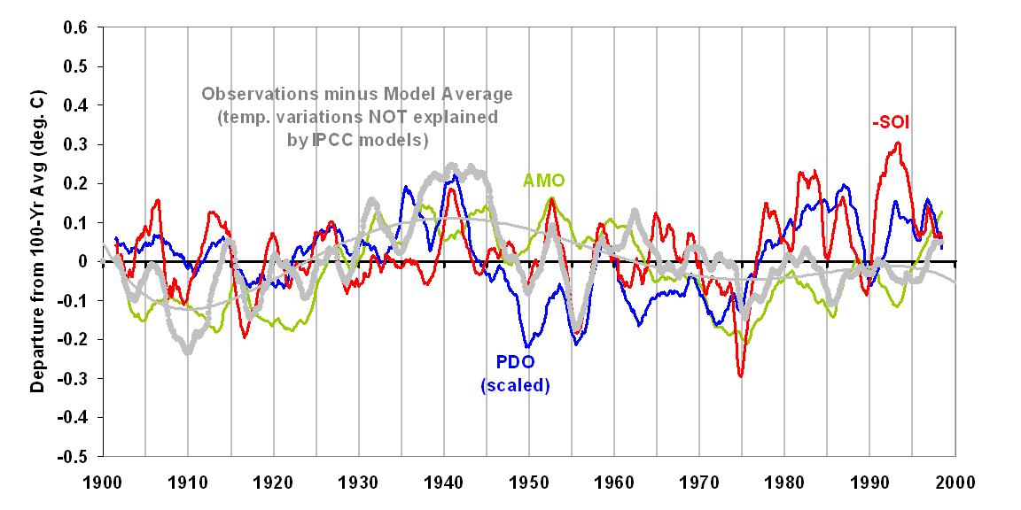
The next chart shows the difference between the two curves in the previous chart, that is, the 20th Century temperature variability the models have not, in an average sense, been able to explain. Also shown are three known modes of natural variability: the Pacific Decadal Oscillation (PDO, in blue); the Atlantic Multidecadal Oscillation (AMO, in green); and the negative of the Southern Oscillation Index (SOI, in red). The SOI is a measure of El Nino and La Nina activity. All three climate indicies have been scaled so that their net amount of variability (standard deviation) matches that of the “unexplained temperature” curve.

As can be seen, the three climate indices all bear some level of resemblance to the unexplained temperature variability in the 20th Century.

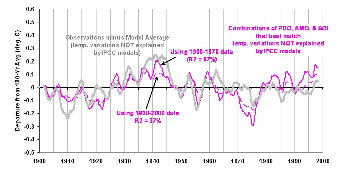
An optimum linear combination of the PDO, AMO, and SOI that best matches the models’ “unexplained temperature variability” is shown as the dashed magenta line in the next graph. There are some time lags included in this combination, with the PDO preceding temperature by 8 months, the SOI preceding temperature by 4 months, and the AMO having no time lag.

This demonstrates that, at least from an empirical standpoint, there are known natural modes of climate variability that might explain at least some portion of the temperature variability seen during the 20th Century. If we exclude the post-1970 data from the above analysis, the best combination of the PDO, AMO, and SOI results in the solid magenta curve. Note that it does a somewhat better job of capturing the warmth around 1940.

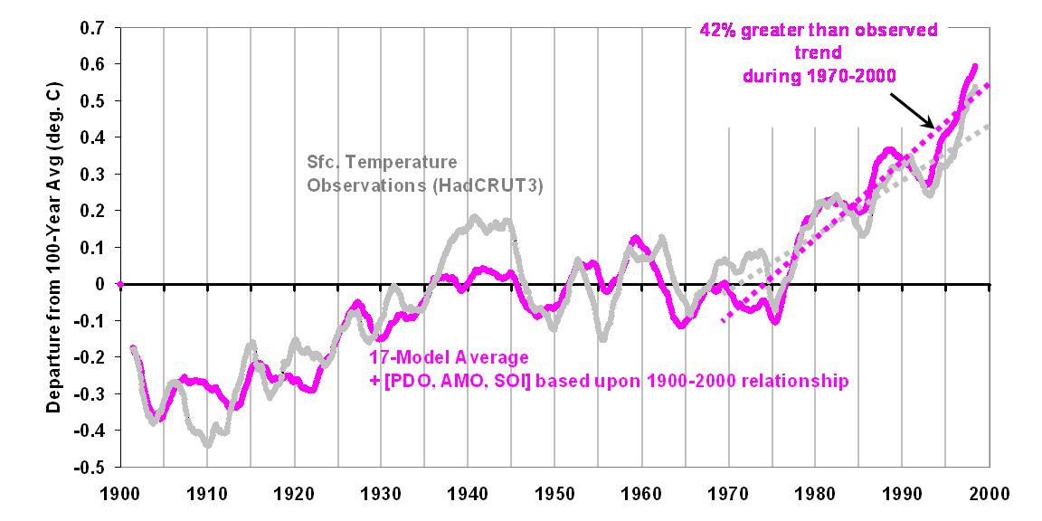
Now, let’s add this natural component in with the original model curve we saw in the first graph, first based upon the full 100 years of overlap:

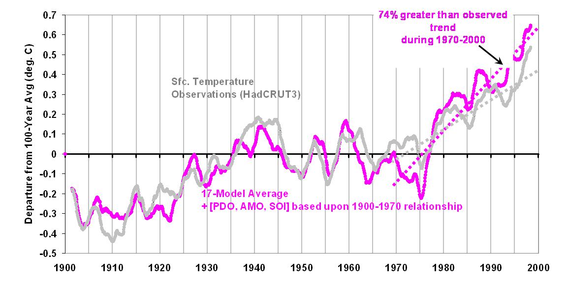
We now find a much better match with the observed temperature record. But we see that the post-1970 warming produced by the combined physical-statistical model tends to be over-stated, by about 40%. If we use the 1900 to 1970 overlap to come up with a natural variability component, the following graph shows that the post-1970 warming is overstated by even more: 74%.

Interpretation
What I believe this demonstrates is that after known, natural modes of climate variability are taken into account, the primary period of supposed CO2-induced warming during the 20th Century – that from about 1970 onward – does not need as strong a CO2-warming effect as is programmed into the average IPCC climate model. This is because the natural variability seen BEFORE 1970 suggests that part of the warming AFTER 1970 is natural! Note that I have deduced this from the IPCC’s inherent admission that they can not explain all of the temperature variability seen during the 20th Century.

The Logical Absurdity of Some Climate Sensitivity Arguments
This demonstrates one of the absurdities (Dick Lindzen’s term, as I recall) in the way current climate change theory works: For a given observed temperature change, the smaller the forcing that caused it, the greater the inferred sensitivity of the climate system. This is why Jim Hansen believes in catastrophic global warming: since he thinks he knows for sure that a relatively tiny forcing caused the Ice Ages, then the greater forcing produced by our CO2 emissions will result in even more dramatic climate change!

But taken to its logical conclusion, this relationship between the strength of the forcing, and the inferred sensitivity of the climate system, leads to the absurd notion that an infinitesimally small forcing causes nearly infinite climate sensitivity(!) As I have mentioned before, this is analogous to an ancient tribe of people thinking their moral shortcomings were responsible for lightning, storms, and other whims of nature.

This absurdity is avoided if we simply admit that we do not know all of the natural forcings involved in climate change. And the greater the number of natural forcings involved, then the less we have to worry about human-caused global warming.

The IPCC, though, never points out this inherent source of bias in its reports. But the IPCC can not admit to scientific uncertainty…that would reduce the chance of getting the energy policy changes they so desire.

One of the great things about the internet is people can post anything they want, no matter how stupid, and lots of people who are incapable of critical thought will simply accept it.

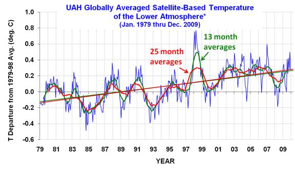
I’m getting emails from people who have read blog postings accusing me of “hiding the increase” in global temperatures when I posted our most recent (Dec. 2009) global temperature update. In addition to the usual monthly temperature anomalies on the graph, for many months I have also been plotting a smoothed version, with a running 13 month average. The purpose of such smoothing is to better reveal longer-term variations, which is how “global warming” is manifested.

But on the latest update, I switched from 13 months to a running 25 month average instead. It is this last change which has led to accusations that I am hiding the increase in global temperatures. Well, here’s a plot with both running averages in addition to the monthly data. I’ll let you decide whether I have been hiding anything:

Note how the new 25-month smoother minimizes the warm 1998 temperature spike, which is the main reason why I switched to the longer averaging time. If anything, this ‘hides the decline’ since 1998…something I feared I would be accused of for sure after I posted the December update.

But just the opposite has happened, with accusations I have hidden the increase. Go figure.

I’m always searching for better and simpler ways to explain the reason why I believe climate researchers have overestimated the sensitivity of our climate system to increasing carbon dioxide concentrations in the atmosphere.

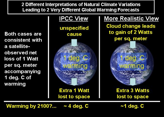
What follows is a somewhat different take than I’ve used in the past. In the following cartoon, I’ve illustrated 2 different ways to interpret a hypothetical (but realistic) set of satellite observations that indicate (1) warming of 1 degree C in global average temperature, accompanied by (2) an increase of 1 Watt per sq. meter of extra radiant energy lost by the Earth to space.

The ‘consensus’ IPCC view, on the left, would be that the 1 deg. C increase in temperature was the cause of the 1 Watt increase in the Earth’s cooling rate. If true, that would mean that a doubling of atmospheric carbon dioxide by late in this century (a 4 Watt decrease in the Earth’s ability to cool) would eventually lead to 4 deg. C of global warming. Not good news.

But those who interpret satellite data in this way are being sloppy. For instance, they never bother to investigate exactly WHY the warming occurred in the first place. As shown on the right, natural cloud variations can do the job quite nicely. To get a net 1 Watt of extra loss you can (for instance) have a gain of 2 Watts of forcing from the cloud change causing the 1 deg. C of warming, and then a resulting feedback response to that warming of an extra 3 Watts.

The net result still ends up being a loss of 1 extra Watt, but in this scenario, a doubling of CO2 would cause little more than 1 deg. C of warming since the Earth is so much more efficient at cooling itself in response to a temperature increase.

Of course, you can choose other combinations of forcing and feedback, and end up deducing just about any amount of future warming you want. Note that the major uncertainty here is what caused the warming in the first place. Without knowing that, there is no way to know how sensitive the climate system is.

And that lack of knowledge has a very interesting consequence. If there is some forcing you are not aware of, you WILL end up overestimating climate sensitivity. In this business, the less you know about how the climate system works, the more fragile the climate system looks to you. This is why I spend so much time trying to separately identify cause (forcing) and effect (feedback) in our satellite measurements of natural climate variability.

As a result of this inherent uncertainty regarding causation, climate modelers are free to tune their models to produce just about any amount of global warming they want to. It will be difficult to prove them wrong, since there is as yet no unambiguous interpretation of the satellite data in this regard. They can simply assert that there are no natural causes of climate change, and as a result they will conclude that our climate system is precariously balanced on a knife edge. The two go hand-in-hand.

Their science thus enters the realm of faith. Of course, there is always an element of faith in scientific inquiry. Unfortunately, in the arena of climate research the level of faith is unusually high, and I get the impression most researchers are not even aware of its existence.

Last year I posted an analysis of satellite observations of the 2007-08 global cooling event, showing evidence that it was due to a natural increase in low cloud cover. Here I will look at the bigger picture of what how the satellite-observed variations in Earth’s radiative budget compare to that expected from increasing carbon dioxide. Is there something that we can say about the relative roles of nature versus humanity based upon the evidence?

What we will find is evidence consistent with natural cloud variations being the dominant source of climate variability since 2000.

CERES Observations of Global Energy Budget Changes
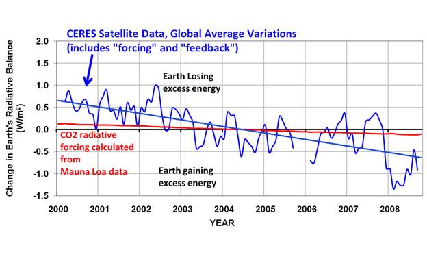
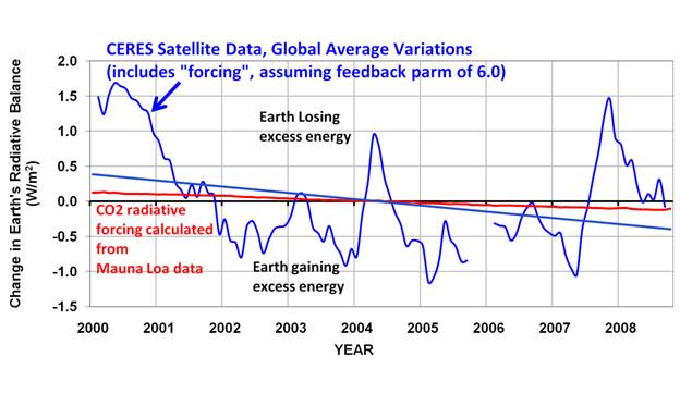
The following graph shows the variations in the Earth’s global-average radiative energy balance as measured by the CERES instrument on NASA’s Terra satellite. These are variations in the imbalance between absorbed sunlight and emitted infrared radiation, the most fundamental quantity associated with global warming or global cooling. Also show (in red) are theoretically calculated changes in radiative forcing from increasing carbon dioxide as measured at Mauna Loa.

Since there is some uncertainty in the absolute accuracy of the CERES measurements, where one puts the zero line is also somewhat uncertain. Therefore, it’s the variations since 2000 which are believed to be pretty accurate, and the exact dividing line between Earth gaining energy and Earth losing energy is uncertain. Significantly, all of the downward trend is in the reflected sunlight portion, not the infrared portion of the variations. We similarly can not reference where the zero line should be for the CO2 forcing, but the reasons for this are more complex and I will not address them here.

In order to compare the variations in the CO2 forcing (in red) to the satellite observations, we need to account for the fact that the satellite observes forcing and feedback intermingled together. So, let’s remove a couple of estimates of feedback from the satellite measurements to do a more direct comparison.

Inferred Forcing Assuming High Climate Sensitivity (IPCC View)
Conceptually, the variations in the Earth’s radiative imbalance are a mixture of forcing (e.g. increasing CO2; clouds causing temperature changes), and feedback (e.g. temperature changes causing cloud changes). We can estimate the forcing part by subtracting out the feedback part.

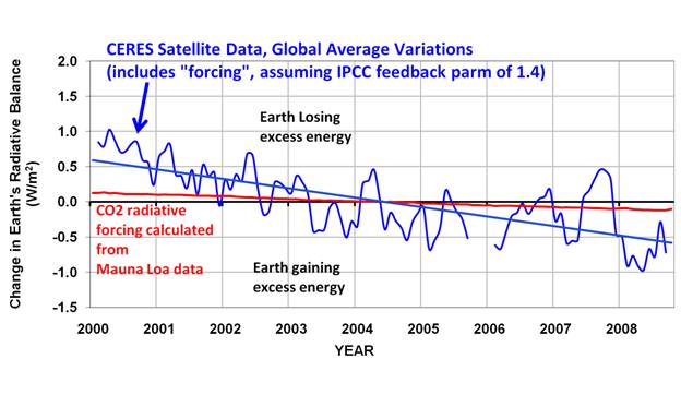
First, let’s assume that the IPCC is correct that climate sensitivity is pretty high. In the following chart I have subtracted out an estimate of the feedback portion of the CERES measurements based upon the IPCC 20-model average feedback parameter of 1.4 W m^-2 K^-1 times the satellite AMSU-measured tropospheric temperature variations

As can be seen, the long-term trend in the CERES measurements is much larger than can be accounted for by increasing carbon dioxide alone, which is presumably buried somewhere in the satellite-measured signal. In fact, the satellite observed trend is in the reflected sunlight portion, not the infrared as we would expect for increasing CO2 (not shown).

Inferred Forcing Assuming Low Climate Sensitivity (“Skeptical” View)
There has been some published evidence (our 2007 GRL paper, Lindzen & Choi’s 2009 paper) to suggest the climate system is quite insensitive. Based upon that evidence, if we assume a net feedback parameter of 6 W m^-2 K^-1 is operating during this period of time, then removing that feedback signal using AMSU channel 5 yields the following history of radiative forcing:

As can be seen, the relative size of the natural forcings become larger since more forcing is required to cause the same temperature changes when the feedback fighting it is strong. Remember, the NET feedback (including the direct increase in emitted IR) is always acting against the forcing…it is the restoring force for the climate system.

What this Might Mean for Global Warming
The main point I am making here is that, no matter whether you assume the climate system is sensitive or insensitive, our best satellite measurements suggest that the climate system is perfectly capable of causing internally-generated radiative forcing larger than the “external” forcing due to increasing atmospheric carbon dioxide concentrations. Low cloud variations are the most likely source of this internal radiative forcing. It should be remembered that the satellite data are actually measured, whereas the CO2 forcing (red lines in the above graphs) is so small that it can only be computed theoretically.

The satellite observed trend toward less energy loss (or, if you prefer, more energy gain) is interesting since there was no net warming observed during this time. How could this be? Well, the satellite observed trend must be due to forcing only since there was no warming or cooling trend during this period for feedback to act upon. And the lack of warming from this substantial trend in the forcing suggests an insensitive climate system.

If one additionally entertains the possibility that there is still considerable “warming still in the pipeline” left from increasing CO2, as NASA’s Jim Hansen claims, then the need for some natural cooling mechanism to offset and thus produce no net warming becomes even stronger. Either that, or the climate system is so insensitive to increasing CO2 that there is essentially no warming left in the pipeline to be realized. (The less sensitive the climate system, the faster it reaches equilibrium when forced with a radiative imbalance.)

Any way you look at it, the evidence for internally-forced climate change is pretty clear. Based upon this satellite evidence alone, I do not see how the IPCC can continue to ignore internally-forced variations in the climate system. The evidence for its existence is there for all to see, and in my opinion, the IPCC’s lack of diagnostic skill in this matter verges on scientific malpractice.

I am still receiving questions about the method by which the satellite microwave measurements are calibrated to get atmospheric temperatures. The confusion seems to have arisen because Christopher Monckton has claimed that our satellite data must be tied to the surface thermometer data, and after Climategate (as well all know) those traditional measurements have become suspect. So, time for a little tutorial.

NASA’S AQUA SATELLITE
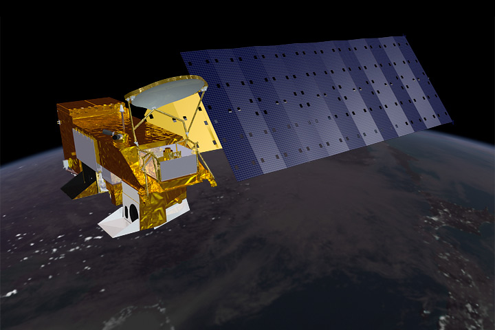
The UAH global temperatures currently being produced come from the Advanced Microwave Sounding Unit (AMSU) flying on NASA’s Aqua satellite. AMSU is located on the bottom of the spacecraft (seen below); the AMSR-E instrument that I serve as the U.S. Science Team Leader for is the one on top of the satellite with the big dish.

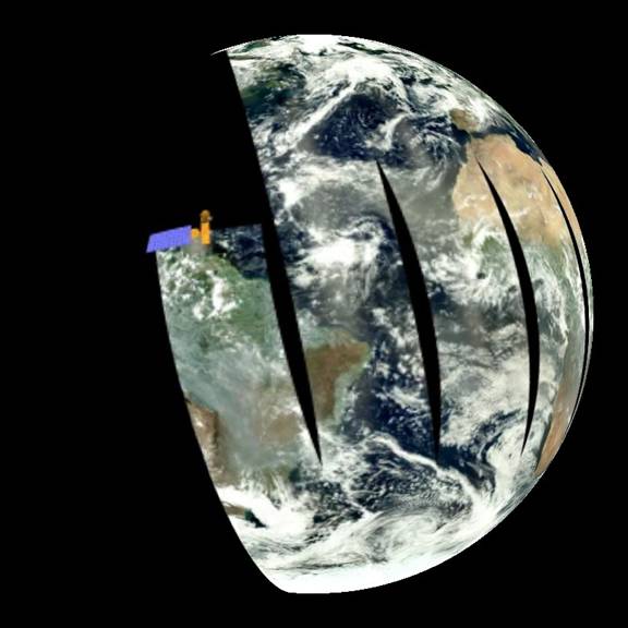
Aqua has been operational since mid-2002, and is in a sun-synchronous orbit that crosses the equator at about 1:30 am and pm local solar time. The following image illustrates how AMSU, a cross-track scanner, continuously paints out an image below the spacecraft (actually, this image comes from the MODIS visible and infrared imager on Aqua, but the scanning geometry is basically the same):

HOW MICROWAVE RADIOMETERS WORK
Microwave temperature sounders like AMSU measure the very low levels of thermal microwave radiation emitted by molecular oxygen in the 50 to 60 GHz oxygen absorption complex. This is somewhat analogous to infrared temperature sounders (for instance, the Atmospheric InfraRed Sounder, AIRS, also on Aqua) which measure thermal emission by carbon dioxide in the atmosphere.

As the instrument scans across the subtrack of the satellite, the radiometer’s antenna views thirty separate ‘footprints’, nominally 50 km in diameter, each over over a 50 millisecond ‘integration time’. At these microwave frequencies, the intensity of thermally-emitted radiation measured by the instrument is directly proportional to the temperature of the oxygen molecules. The instrument actually measures a voltage, which is digitized by the radiometer and recorded as a certain number of digital counts. It is those digital counts which are recorded on board the spacecraft and then downlinked to satellite tracking stations in the Arctic.

HOW THE DATA ARE CALIBRATED TO TEMPERATURES
Now for the important part: How are these instrument digitized voltages calibrated in terms of temperature?

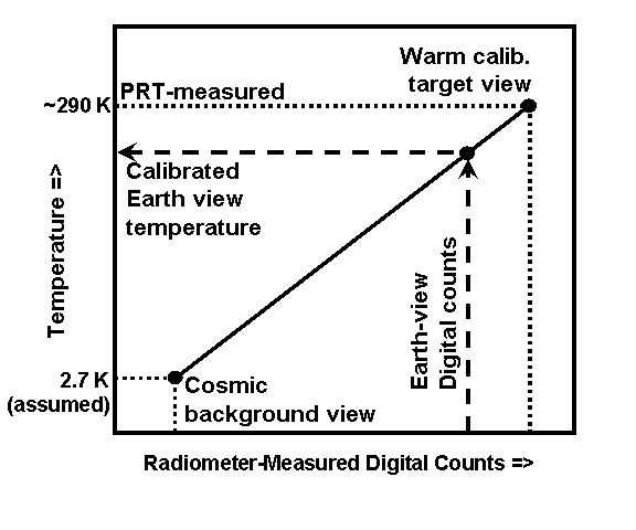
Once every Earth scan, the radiometer antenna looks at a “warm calibration target” inside the instrument whose temperature is continuously monitored with several platinum resistance thermometers (PRTs). PRTs work somewhat like a thermistor, but are more accurate and more stable. Each PRT has its own calibration curve based upon laboratory tests.

The temperature of the warm calibration target is allowed to float with the rest of the instrument, and it typically changes by several degrees during a single orbit, as the satellite travels in and out of sunlight. While this warm calibration point provides a radiometer digitized voltage measurement and the temperature that goes along with it, how do we use that information to determine what temperatures corresponds to the radiometer measurements when looking at the Earth?

A second calibration point is needed, at the cold end of the temperature scale. For that, the radiometer antenna is pointed at the cosmic background, which is assumed to radiate at 2.7 Kelvin degrees. These two calibration points are then used to interpolate to the Earth-viewing measurements, which then provides the calibrated “brightness temperatures”. This is illustrated in the following graph:

The response of the AMSU is slightly non-linear, so the calibration curve in the above graph actually has slight curvature to it. Back when all we had were Microwave Sounding Units (MSU), we had to assume the instruments were linear due to a lack of sufficient pre-launch test data to determine their nonlinearity. Because of various radiometer-related and antenna-related factors, the absolute accuracy of the calibrated Earth-viewing temperatures are probably not much better than 1 deg. C. While this sounds like it would be unusable for climate monitoring, the important thing is that the instruments be very stable over time; an absolute accuracy error of this size is irrelevant for climate monitoring, as long as sufficient data are available from successive satellites so that the newer satellites can be calibrated to the older satellites’ measurements.

WHAT LAYERS OF THE ATMOSPHERE ARE MEASURED?
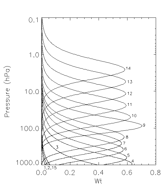
For AMSU channel 5 that we use for tropospheric temperature monitoring, that brightness temperature is very close to the vertically-averaged temperature through a fairly deep layer of the atmosphere. The vertical profiles of each channel’s relative sensitivity to temperature (‘weighting functions’) are shown in the following plot:

These weighting functions are for the nadir (straight-down) views of the instrument, and all increase in altitude as the instrument scans farther away from nadir. AMSU channel 5 is used for our middle tropospheric temperature (MT) estimate; we use a weighted difference between the various view angles of channel 5 to probe lower in the atmosphere, which a fairly sharp weighting function which is for our lower-tropospheric (LT) temperature estimate. We use AMSU channel 9 for monitoring of lower stratospheric (LS) temperatures.

For those channels whose weighting functions intersect the surface, a portion of the total measured microwave thermal emission signal comes from the surface. AMSU channels 1, 2, and 15 are considered “window” channels because the atmosphere is essentially clear, so virtually all of the measured microwave radiation comes from the surface. While this sounds like a good way to measure surface temperature, it turns out that the microwave ’emissivity’ of the surface (it’s ability to emit microwave energy) is so variable that it is difficult to accurately measure surface temperatures using such measurements. The variable emissivity problem is the smallest for well-vegetated surfaces, and largest for snow-covered surfaces. While the microwave emissivity of the ocean surfaces around 50 GHz is more stable, it just happens to have a temperature dependence which almost exactly cancels out any sensitivity to surface temperature.

POST-PROCESSING OF DATA AT UAH
The millions of calibrated brightness temperature measurements are averaged in space and time, for instance monthly averages in 2.5 degree latitude bands. I have FORTRAN programs I have written to do this. I then pass the averages to John Christy, who inter-calibrates the different satellites’ AMSUs during periods when two or more satellites are operating (which is always the case).

The biggest problems we have had creating a data record with long-term stability is orbit decay of the satellites carrying the MSU and AMSU instruments. Before the Aqua satellite was launched in 2002, all other satellites carrying MSUs or AMSUs had orbits which decayed over time. The decay results from the fact that there is a small amount of atmospheric drag on the satellites, so they very slowly fall in altitude over time. This leads to 3 problems for obtaining a stable long-term record of temperature.

(1) Orbit Altitude Effect on LT The first is a spurious cooling signal in our lower tropospheric (LT) temperature product, which depends upon differencing measurements at different view angles. As the satellite falls, the angle at which the instrument views the surface changes slightly. The correction for this is fairly straightforward, and is applied to both our dataset and to the similar datasets produced by Frank Wentz and Carl Mears at Remote Sensing Systems (RSS). This adjustment is not needed for the Aqua satellite since it carries extra fuel which is used to maintain the orbit.

(2) Diurnal Drift Effect The second problem caused by orbit decay is that the nominal local observation time begins to drift. As a result, the measurements can increasingly be from a warmer or cooler time of day after a few years on-orbit. Luckily, this almost always happened when another satellite operating at the same time had a relatively stable observation time, allowing us to quantify the effect. Nevertheless, the correction isn’t perfect, and so leads to some uncertainty. [Instead of this empirical correction we make to the UAH products, RSS uses the day-night cycle of temperatures created by a climate model to do the adjustment for time-of-day.] This adjustment is not necessary for the Aqua AMSU.

(3) Instrument Body Temperature Effect. As the satellite orbit decays, the solar illumination of the spacecraft changes, which then can alter the physical temperature of the instrument itself. For some unknown reason, it turns out that most of the microwave radiometers’ calibrated Earth-viewing temperatures are slightly influenced by the temperature of the instrument itself…which should not be the case. One possibility is that the exact microwave frequency band which the instrument observes at changes slightly as the instrument warms or cools, which then leads to weighting functions that move up and down in the atmosphere with instrument temperature. Since tropospheric temperature falls off by about 7 deg. C for every 1 km in altitude, it is important for the ‘local oscillators’ governing the frequency band sensed to be very stable, so that the altitude of the layer sensed does not change over time. This effect is, once again, empirically removed based upon comparisons to another satellite whose instrument shows little or no instrument temperature effect. The biggest concern is the long-term changes in instrument temperature, not the changes within an orbit. Since the Aqua satellite does not drift, the solar illumination does not change and and so there is no long-term change in the instrument’s temperature to correct for.

One can imagine all kinds of lesser issues that might affect the long-term stability of the satellite record. For instance, since there have been ten successive satellites, most of which had to be calibrated to the one before it with some non-zero error, there is the possibility of a small ‘random walk’ component to the 30+ year data record. Fortunately, John Christy has spent a lot of time comparing our datasets to radiosonde (weather balloon) datasets, and finds very good long-term agreement.

YR MON GLOBE NH SH TROPICS
2009 1 +0.304 +0.443 +0.165 -0.036
2009 2 +0.347 +0.678 +0.016 +0.051
2009 3 +0.206 +0.310 +0.103 -0.149
2009 4 +0.090 +0.124 +0.056 -0.014
2009 5 +0.045 +0.046 +0.044 -0.166
2009 6 +0.003 +0.031 -0.025 -0.003
2009 7 +0.411 +0.212 +0.610 +0.427
2009 8 +0.229 +0.282 +0.177 +0.456
2009 9 +0.422 +0.549 +0.294 +0.511
2009 10 +0.286 +0.274 +0.297 +0.326
2009 11 +0.497 +0.422 +0.572 +0.495
2009 12 +0.280 +0.318 +0.242 +0.503

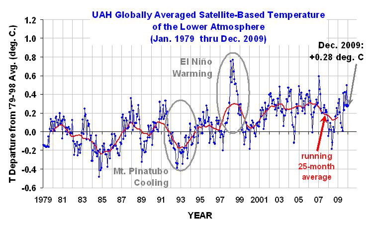
The global-average lower tropospheric temperature anomaly fell back to the October level of +0.28 deg. C in December. The tropics continue warm from El Nino conditions there, while the NH and SH extratropics anomalies cooled from last month. While the large amount of year-to-year variability in global temperatures seen in the above plot makes it difficult to provide meaningful statements about long-term temperature trends in the context of global warming, the running 25-month average suggests there has been no net warming in the last 11 years or so.

[NOTE: These satellite measurements are not calibrated to surface thermometer data in any way, but instead use on-board redundant precision platinum resistance thermometers carried on the satellite radiometers.]