Monthly Archives: March 2018

U.S. chance of Tiangong-1 sighting now less than 2%

The latest Aerospace Corp. prediction of the reentry time for the Chinese Space Station Tiangong-1 is now 3:30 p.m. CDT (plus or minus 8 hours) on Sunday, April 1. As reentry approaches, the predictions will get better, and the potential paths of the satellite will be narrowing.

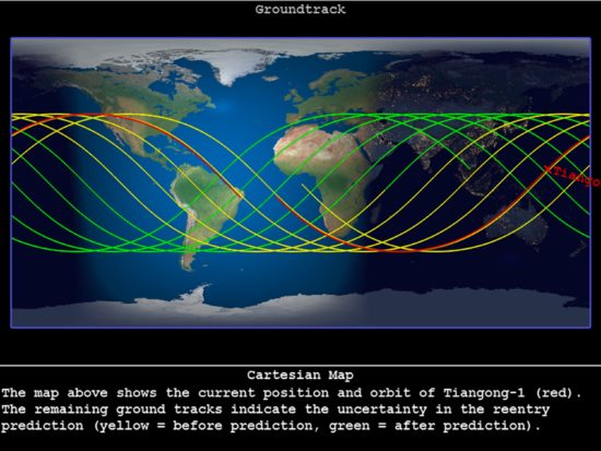
The latest potential paths of reentry look like this:

Potential Tiangong-1 reentry orbital paths on April 1 2018 (Aerospace Corp.)

The paths over the U.S. are morning paths, and would be quite early in the time window of reentry. The total time these orbits are visible from the contiguous U.S. is only about 25 minutes (you could see the satellite burning up as far as 400 miles away from these paths, assuming no clouds are in the way). That is only 2.6 percent of the total time of the reentry window (16 hours), so given the the fact the U.S. paths are quite early in the window (and thus lower probability), I’d say the chances of anyone in the U.S. getting to see the fireworks show is less than 2%. Once you factor in cloud cover, it’s probably more like 1%.

Of course, we always knew the probability was very small.

And I think Michigan can now deactivate their Emergency Operations Center.

But, if you are feeling lucky and live within a few hundred miles of one of the paths show in the above graphic, I suggest visiting heavens-above.com, (1) enter your location (or nearest city), (2) click on “Tiangong-1”, and (3) change from “Visible only” to “All”, to see exactly what time(s) the satellite will be passing near you. Click on one of those times to see the path it will be making across the sky.

Lord Monckton Responds

NOTE: In fairness to Lord Monckton, I have accepted his request to respond to my post where I criticized his claim than an “elementary error of physics” could be demonstrated on the part of climate modelers. While Christopher & I are in agreement that the models produce too much warming, we disagree on the reasons why. From what I can tell, Christopher claims that climatologists have assumed the theoretical 255K average global surface temperature in the absence of the greenhouse effect would actually induce a feedback response; I disagree… 255K is the theoretical, global average temperature of the Earth without greenhouse gases but assuming the same solar insolation and albedo. It has no feedback response because it is a pure radiative equilibrium calculation. Besides, the climate models do not depend upon that theoretical construct anyway; it has little practical value — and virtually no quantitative value –other than in conceptual discussions (how could one have clouds without water vapor? How could a much colder Earth have no more ice cover than today?). But I will let the reader decide whether his arguments have merit. I do think the common assumption that the climate system was in equilibrium in the mid-1800s is a dubious one, and I wish we could attack that, instead, because if some of the warming since the 1800s was natural (which I believe is likely) it would reduce estimates of climate sensitivity to increasing carbon dioxide even further.

Of ZOD and NOGs

By Christopher Monckton of Brenchley

Roy Spencer has very kindly allowed me to post up this reply to his interesting posting about my team’s discussion of a large error we say we have found in climatological physics.

The error arises from the fact that climate models are calibrated by reference to past climate. They have to explain why the world in, say, 1850, was 32 K warmer than the 255 K that would have prevailed that year (assuming today’s insolation and an albedo of about 0.3), in the absence of the naturally-occurring, non-condensing greenhouse gases (NOGS).

Till now, it has generally been assumed that between a third and a quarter of that 32 K warming is directly forced by the presence of the NOGS, and that between two-thirds and three-quarters is a feedback response to the directly-forced warming from the NOGS.

That gives a feedback fraction of 2/3 to 3/4, or 0.67 to 0.75. The feedback fraction is simply the fraction of final or equilibrium temperature that constitutes the feedback response to the directly-forced warming.

Roy is quite right to point out that the general-circulation models do not use the concept of feedback directly. However, there is a handy equation, with the clunky name zero-dimensional-model equation (lets call it ZOD) that allows us to diagnose what equilibrium temperature the models would predict.

All we need to know to diagnose the equilibrium temperature the models would be expected to predict is the reference temperature, here the 255 K emission temperature, and the feedback fraction.

ZOD works also for changes in temperature rather than entire temperatures. The reason is that a temperature feedback is a temperature response induced by a temperature or temperature change.

If a feedback is present in a dynamical system (that’s a mathematically-describable object that changes its state over time, such as the climate), that feedback does not distinguish between the initial entire temperature (known to feedback-analysis geeks as the input signal) and any change in that temperature (the direct gain), such as a directly-forced increase owing to the presence of NOGS.

We say that climatology errs in assuming that the input signal (the 255 K emission temperature that would prevail at the surface in the absence of greenhouse gases) does not induce a feedback response, but that the additional 8 Kelvin of warming directly forced by the presence of the NOGS somehow, as if by magic, induces a feedback response and not just any old feedback response, but a temperature of 24 K, three times the direct warming that induced it.

Now, here’s the question for anyone who thinks climatology has gotten this right. By what magical process waving a wand, scattering stardust, casting runes, reading tea-leaves, pick a card, any card do the temperature feedbacks in the climate distinguish between the input signal of 255 K and the direct gain of 8 K in deciding whether to respond?

Do the feedbacks gather around, have a beer and take a vote? OK, boys, lets go on strike until the surface temperature exceeds 255 K, and lets go to work in a big way then, but only in response to the extra 8 K of temperature from our good mates the NOGs?

Of course not. If a feedback process subsists in a dynamical object, it will respond not only to what the feedback geeks call the direct gain but also to the input signal. Why on Earth would feedbacks refuse to deliver any response at all to 255 K of emission temperature but then suddenly deliver a whopper of a 24 K response to just 8 K of further temperature?

Roy’s difficulty in accepting that the emission temperature induces a feedback response is that it is not a forcing. Of course it isn’t. Emission temperature, as its name suggests, is a temperature, denominated in Kelvin, not a forcing (a change in radiative flux density denominated in Watts per square meter).

But what is a temperature feedback? The clue is in the name on the tin. A temperature feedback is a feedback to temperature, not to a forcing. It is itself a forcing, this time denominated in Watts per square meter per Kelvin of the temperature (or temperature change) that induced it.

A temperature feedback just doesn’t care whether it is responding to an initial temperature, or to a subsequent change in temperature driven by a forcing such as that from the presence of the NOGs.

Take the Earth in 1850, but without greenhouse gases, and yet preserving today’s insolation and albedo. The reason for this rather artificial construct is that that’s the way climatology determines the influence of feedbacks, by comparing like with like. The ice, clouds and sea have much the same extents as today, so the thought experiment says.
And that means there are feedbacks. Specifically, the water-vapor feedback somewhat offset by the lapse-rate feedback, the surface albedo feedback, and the cloud feedbacks.
Those feedbacks respond to temperature. Is there one? Yes. There is a temperature of 255 K. At this stage in the calculation, we don’t have much of an idea of how much the feedback response to 255 K of temperature would be.

Lets press ahead and bring on the NOGS. Up goes the temperature by a directly-forced 8 K, from 255 K to 263 K, or thereabouts.

What’s the equilibrium temperature in this experiment? Its simply the actual, measured temperature in 1850: namely, around 287 K. The climate is presumed to have been in equilibrium then.

Now we have all we need to deploy the ZOD to diagnose approximately what the feedback fraction would be in the models, provided that, as in this experiment, they took account of the fact that the emission temperature as well as well as the NOGs induces a feedback response.

The ZOD is a really simple equation. If, as here, we have some idea of the reference temperature (in this case, 263 K) and the equilibrium temperature (287 K), the feedback fraction is simply 1 minus the ratio of emission temperature to equilibrium temperature, thus: 1 – 263/287. That works out at 0.08, and not, as now, 0.67 or 0.75.

Armed with the approximate value of the feedback fraction, we can use the ZOD to work out the Charney sensitivity (i.e., equilibrium sensitivity to doubled CO2) if the models were to take account of the fact that feedbacks will respond just as enthusiastically to the emission temperature as to the small change in that temperature forced by the presence of the NOGS.

The models current estimate of reference sensitivity to doubled CO2 is 1.1 K. Using their current estimate of the feedback fraction, 0.67, the ZOD tells us Charney sensitivity would be 1.1/(1 – 0.67), or a heftyish 3.3 K. That’s the official mid-range estimate.

But with our corrected approximation to the feedback fraction, Charney sensitivity would be 1.1/(1 – 0.08), or only 1.2 K. End of global warming problem.

What of Roy’s point that the models don’t explicitly use the ZOD? The models have been tuned to assume that two-thirds to three-quarters of the 32 K difference between emission temperature and real-world temperature in 1850 is accounted for by feedback responses to the 8 K directly forced warming from the NOGs.

The models are also told that there is no feedback response to the 255 K emission temperature, even though it is 32 times bigger than the 8 K warming from the NOGs.

So they imagine, incorrectly, that Charney sensitivity is almost three times the value that they would find if the processes by which they represent what we are here calling feedbacks had been adjusted to take account of the fact that feedbacks respond to any temperature, whether it be the entire original temperature or some small addition to it.

Mainstream climate science thus appeared to us to be inconsistent with mainstream science. So we went to a government laboratory and said, Build us an electronic model of the climate, and do the following experiment. Assume that the input signal is 255 K. Assume that there are no greenhouse gases, so that the value of the direct-gain factor in the gain block is unity [feedback geek-speak, but they knew what we meant]. Assume that the feedback fraction is 0.1. And tell us what the output signal would be.

Now, climatology would say that, in the absence of any forcings from the greenhouse gases, the output signal would be exactly the same as the input signal: 255 K. But we said to the government lab, We think the answer will be 283 K.

So the lab built the test circuit, fed in the numbers, and simply measured the output, and behold, it was 283 K. They weren’t at all surprised, and nor were we. For ZOD said 255/(1 – 0.1) = 283.

That’s it, really. But our paper is 7500 words long, because we have had to work so hard to nail shut the various rat-holes by which climatologists will be likely to try to scurry away.

Will it pass peer review? Time will tell. But we have the world’s foremost expert in optical physics and the world’s foremost expert in the application of feedback math to climate on our side.

Above all, we have ZOD on our side. ZOD gives us a very simple way of working out what warming the models would predict if they did things right. We calibrated ZOD by feeding in the official CMIP5 models values of the reference temperature and of the feedback fraction, and we obtained the official interval of Charney sensitivities that the current models actually predict. ZOD works.

We went one better. We took IPCC’s mid-range estimate of the net forcing from all anthropogenic sources from 1850-2011 and worked out that that implied a reference sensitivity over that period of 0.72 K. But the actual warming was 0.76 K, and that’s near enough the equilibrium warming (it might be a little higher, owing to delays caused by the vast heat-sink that is the ocean).

And ZOD said that the industrial-era feedback fraction was 1 – 0.72/0.76, or 0.05. That was very close to the pre-industrial feedback fraction 0.08, but an order of magnitude smaller than the official estimates, 0.67-0.75.

Or ZOD can do it the other way about. If the feedback fraction is really 0.67, as the CMIP5 models think, then the equilibrium warming from 1850-2011 would not be the measured 0.76 K: it would be 0.72/(1 – 0.67) = 2.2 K, almost thrice what was observed.

Does ocean overturning explain that discrepancy? Well, we know from the pre-industrial experiment, in which ocean overturning is inapplicable, that the feedback fraction is about 0.08. And there’s not likely to be all that much difference between the pre-industrial and industrial-era values of the feedback fraction.

ZOD, therefore, works as a diagnostic tool. And ZOD tells us Charney sensitivity to doubled CO2 will be only 1.2 K, plus or minus not a lot. Game over.

Or so we say.

Climate F-Words

President Trump explaining climate change terminology.


A recent article by Lord Christopher Monckton over at WUWT argues that there has been an “elementary error of physics” that has led to climate sensitivity being overestimated by about a factor of 2.

I agree with the conclusion but not the reason why. It is already known from the work of Otto et al. (2013), Lewis & Curry (2015) and others that the climate system (including the deep oceans) has warmed by an amount that suggests a climate sensitivity only about half of what the models produce (AR5 models warm by an average of 3.4 deg. C in response to a doubling of CO2).

But the potential reasons why are many, and as far as I can tell not dependent upon Christopher’s arguments. For those who don’t know, Lord Monckton is a pretty talented mathematician. However, like others I have encountered over the years, I believe he errs in his assumptions about how the climate research community uses — and does or does not depend upon — the concept of feedback in climate modeling.

You Don’t Have to Use F-Words

I’ve been told that the feedback concept used by climate researchers is a very poor analog for feedbacks in electrical circuit design. Fine. It doesn’t matter. How modern 3D coupled ocean-atmosphere climate models work does not depend upon the feedback concept.

What they DO depend upon is energy conservation: If the system is in energy equilibrium, its average temperature will not change (that’s not precisely true, because it makes little sense energetically to average the temperature of all ocean water with the atmosphere, and there can be energy exchanges between these two reservoirs which have vastly different heat capacities. Chris Essex has written on this). The point is that the total heat content of the system in Joules stays the same unless an energy imbalance occurs. (Temperature is focussed on so intensely because it determines the rate at which the Earth sheds energy to outer space. Temperature stabilizes the climate system.)

The amount of surface temperature change in response to that energy imbalance is, by definition, the climate sensitivity, which in turn depends upon feedback components. You can call the feedbacks anything… maybe “temperature sensitivity parameters” if you wish. Feedback is just a convenient term that quantifies the proportionality between an imposed energy imbalance and the resulting temperature change response, whether it’s for a pot of water on the stove, the climate system, or anything that is initially at a constant temperature but then is forced to change its temperature. Christopher’s claim that the Earth’s effective radiating temperature (ERT) to outer space (around 255 K) itself causes a “feedback” makes no sense to me, because it isn’t (nor does it represent) a “forcing”. Feedbacks, by the climate definition, are only in response to forced departures from energy equilibrium.

The proportionality factor between a forcing (another f-word) and temperature response in climate parlance is called the net feedback parameter, and has units of Watts per sq. meter per deg. C, usually referenced to a surface temperature change. You could come up with a sensitivity parameter for a pot of water on the stove, too. In the climate system the net feedback parameter has components from temperature-dependent changes in clouds, water vapor, etc., as well as the Sigma-T^^4 “Planck” effect that ultimately stabilizes the climate system from experiencing large temperature fluctuations.

Now, in the process of describing climate change in simple terms with such proportionalities between imposed energy imbalance and temperature response, various feedback equations have been published. But NONE of the IPCC models depend upon any formulation of any feedback equation you wish to devise. Neither do they depend upon whether the Earth’s natural greenhouse effect on surface temperature is estimated to be 33 deg. C, or 75 deg. C (Manabe & Strickler, 1964), or any other value. Nor do they depend upon how that 33 deg or 75 deg is apportioned from different components. These are all conceptual constructs which help us understand and discuss the climate system, but the climate models do not depend upon them.

Modern 3D climate models are basically weather forecast models (with an ocean model added) that are run for a hundred years or more of model run time (rather than 3-14 days, which is pretty common for weather forecast models). One of the biggest differences is that climate models have been tuned so that they keep a relatively constant temperature over a long integration, which also means their rates of energy gain (from the sun) and energy loss to outer space are, in the long term, equal. (I question whether they actually conserve energy, but that’s a different discussion).

Once you have a model whose temperature does not drift over time, then you can impose a forcing upon it. All that means is impose an energy imbalance. Once again, it doesn’t matter to the physics what you call it. To change the energy balance, you could increase the solar input. Or, you could reduce the rate of radiative cooling to outer space, e.g. from increasing atmospheric CO2. The point is that forcing is just an imposed energy imbalance, while feedback quantifies how much of a temperature response you will get for a given amount of forcing.

As the climate system warms from an energy imbalance, a wide variety of changes can take place (clouds, water vapor, etc.) which affect how much warming will occur before energy balance is once again restored, and the system stops warming. Those component changes, for better or worse, are called “feedbacks” (e.g. cloud feedback, water vapor feedback). Again, you don’t have to use the f-word. Call it anything you want. Its just a proportionality constant (or not a constant?) that quantitatively relates an energy imbalance to a temperature response.

Nowhere do the IPCC models invoke, use, assume, or otherwise depend upon any feedback equations. Those equations are just greatly simplified approximations that allow us to discuss how the climate system responds to an imposed energy imbalance. If somebody has published a paper that incorrectly explains the climate system with a feedback equation, that does not invalidate the models. There might be many errors in models that cause them to be too sensitive, but how someone misrepresents the model behavior with their favorite feedback equation is that person’s problem… not the model’s problem.

Feedbacks in the IPCC models are diagnosed after the model is run; they are not specified before it is run. Now, it IS true that how some uncertain model processes such as cloud parameterizations are specified will affect the feedbacks, and therefore affect the climate sensitivity of the model. So, I suppose you can say that feedbacks are indirectly imposed upon the models. But there isn’t a feedback factor or feedback equation input into the model.

The ultimate climate sensitivity of the models to an energy imbalance (say, increasing CO2) depends upon how clouds, water vapor, etc., all change with warming in the model in such a way to make the warming either large or small. The equations in the models governing this involve energy and mass conservation, moisture, thermodynamics, dynamics, radiation, etc., along with some crucial approximations for processes which the models cannot resolve (e.g. cloud parameterizations, which will affect cloud feedback) or which we do not even understand well enough to put in the models (e.g. temperature-dependent changes in precipitation efficiency, which will affect water vapor feedback).

But nowhere does the sensitivity of modern 3D climate models depend upon any feedback equations.

Now, if I have misrepresented Lord Monckton’s argument, I apologize. But I am having difficulty determining exactly what his argument is, and how it affects the processes specified in climate models. Maybe someone can help me. We can agree that the models are too sensitive, but we must make sure our arguments for their excessive sensitivity make sense, or we will continue to be dismissed out of hand by the mainstream climate community.

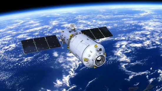
Chinese satellite filled with corrosive fuel will probably hit… the ocean

Oh, boy. If only reporters checked with anyone who knows orbital mechanics before writing stories like this:

Chinese satellite filled with corrosive fuel could hit lower Michigan

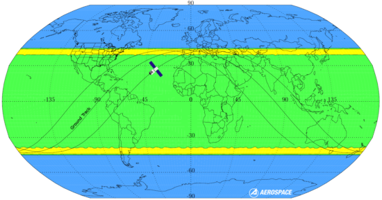
The orbital decay of the Chinese space station Tiangong-1 will lead to its uncontrolled reentry around April. The green and yellow areas on the following map show where the satellite might hit…somewhere:

Now, because of the inclination of the orbit (the highest latitude it reaches), the yellow areas have a higher probability of being hit than the green area…per square mile. But the green area is a whole lot bigger than the yellow area.

As a result, past experience has shown that these satellites usually reenter over the ocean…usually the Pacific. It’s a really big area.

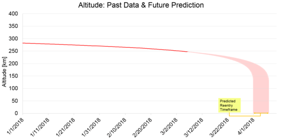
As the satellite falls, it encounters more atmospheric drag (anyone see the movie Gravity?) The resulting enhanced orbital decay then becomes very rapid, and the satellite burns up. But the point at which this happens is unpredictable. If the reentry prediction is off by, say, 50 minutes (a half orbit), the satellite will reenter on the opposite side of the Earth (!)

Here’s a recent reentry window forecast from the Aerospace Corporation…note the window is about 6 days wide. And, again… a 50 minute error in the prediction means the other side of the world:

So, to do a news story that the satellite might hit Lower Michigan… well… that takes an extra dose of either moxey or idiocy.

UAH Global Temperature Update for February, 2018: +0.20 deg. C

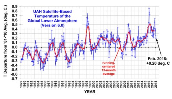
The Version 6.0 global average lower tropospheric temperature (LT) anomaly for February, 2018 was +0.20 deg. C, down a little from the January value of +0.26 deg. C:

Global area-averaged lower tropospheric temperature anomalies (departures from 30-year calendar monthly means, 1981-2010). The 13-month centered average is meant to give an indication of the lower frequency variations in the data; the choice of 13 months is somewhat arbitrary… an odd number of months allows centered plotting on months with no time lag between the two plotted time series. The inclusion of two of the same calendar months on the ends of the 13 month averaging period causes no issues with interpretation because the seasonal temperature cycle has been removed, and so has the distinction between calendar months.

The global, hemispheric, and tropical LT anomalies from the 30-year (1981-2010) average for the last 14 months are:

YEAR MO GLOBE NHEM. SHEM. TROPICS
2017 01 +0.33 +0.31 +0.34 +0.10
2017 02 +0.38 +0.57 +0.19 +0.08
2017 03 +0.23 +0.36 +0.09 +0.06
2017 04 +0.27 +0.28 +0.26 +0.21
2017 05 +0.44 +0.39 +0.49 +0.41
2017 06 +0.21 +0.33 +0.10 +0.39
2017 07 +0.29 +0.30 +0.27 +0.51
2017 08 +0.41 +0.40 +0.42 +0.46
2017 09 +0.54 +0.51 +0.57 +0.54
2017 10 +0.63 +0.66 +0.59 +0.47
2017 11 +0.36 +0.33 +0.38 +0.26
2017 12 +0.41 +0.50 +0.33 +0.26
2018 01 +0.26 +0.46 +0.06 -0.12
2018 02 +0.20 +0.24 +0.15 +0.03

The linear temperature trend of the global average lower tropospheric temperature anomalies from January 1979 through February 2018 remains at +0.13 C/decade.

The UAH LT global anomaly image for February, 2018 should be available in the next few days here.

The new Version 6 files should also be updated in the coming days, and are located here:

Lower Troposphere: http://vortex.nsstc.uah.edu/data/msu/v6.0/tlt/uahncdc_lt_6.0.txt
Mid-Troposphere: http://vortex.nsstc.uah.edu/data/msu/v6.0/tmt/uahncdc_mt_6.0.txt
Tropopause: http://vortex.nsstc.uah.edu/data/msu/v6.0/ttp/uahncdc_tp_6.0.txt
Lower Stratosphere: http://vortex.nsstc.uah.edu/data/msu/v6.0/tls/uahncdc_ls_6.0.txt