After years of dabbling in this issue, John Christy and I have finally submitted a paper to Journal of Applied Meteorology and Climatology entitled, “Urban Heat Island Effects in U.S. Summer Surface Temperature Data, 1880-2015“.

I feel pretty good about what we’ve done using the GHCN data. We demonstrate that, not only do the homogenized (“adjusted”) dataset not correct for the effect of the urban heat island (UHI) on temperature trends, the adjusted data appear to have even stronger UHI signatures than in the raw (unadjusted) data. This is true of both trends at stations (where there are nearby rural and non-rural stations… you can’t blindly average all of the stations in the U.S.), and it’s true of the spatial differences between closely-space stations in the same months and years.

The bottom line is that an estimated 22% of the U.S. warming trend, 1895 to 2023, is due to localized UHI effects.

And the effect is much larger in urban locations. Out of 4 categories of urbanization based upon population density (0.1 to 10, 10-100, 100-1,000, and >1,000 persons per sq. km), the top 2 categories show the UHI temperature trend to be 57% of the reported homogenized GHCN temperature trend. So, as one might expect, a large part of urban (and even suburban) warming since 1895 is due to UHI effects. This impacts how we should be discussing recent “record hot” temperatures at cities. Some of those would likely not be records if UHI effects were taken into account.

Yet, those are the temperatures a majority of the population experiences. My point is, such increasing warmth cannot be wholly blamed on climate change.

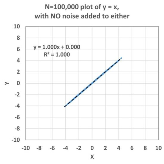
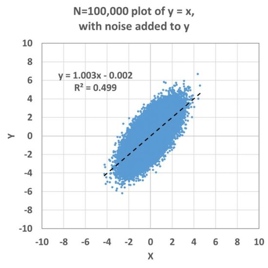
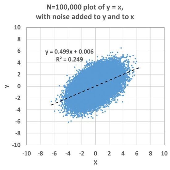
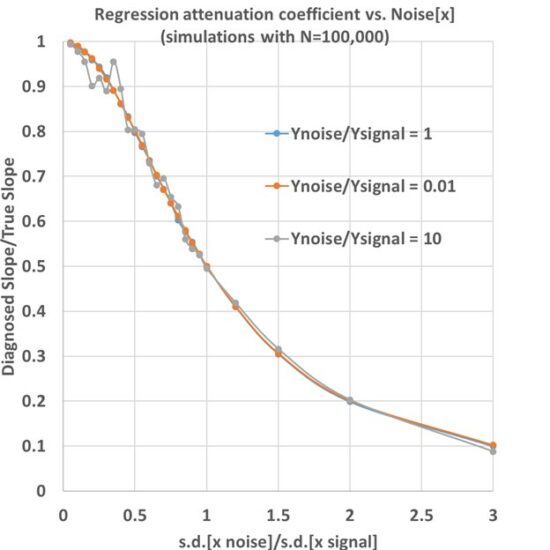
One of the things I struggled with was how to deal with stations having sporadic records. I’ve always wondered if one could use year-over-year changes instead of the usual annual-cycle-an-anomaly calculations, and it turns out you can, and with extremely high accuracy. (John Christy says he did it many years ago for a sparse African temperature dataset). This greatly simplifies data processing, and you can use all stations that have at least 2 years of data.

Now to see if the peer review process deep-sixes the paper. I’m optimistic.

I’m not a statistician, and I am hoping someone out there can tell me where I’m wrong in the assertion represented by the above title. Or, if you know someone expert in statistics, please forward this post to them.

In regression analysis we use statistics to estimate the strength of the relationship between two variables, say X and Y.

Standard least-squares linear regression estimates the strength of the relationship (regression slope “m”) in the equation:

Y = mX + b, where b is the Y-intercept.

In the simplest case of Y = X, we can put in a set of normally distributed random numbers for X in Excel, and the relationship looks like this:

Now, in the real world, our measurements are typically noisy, with a variety of errors in measurement, or variations not due, directly or indirectly, to correlated behavior between X and Y. Importantly, standard least squares regression estimation assumes all of these errors are in Y, and not in X. This issue is seldom addressed by people doing regression analysis.

If we next add an error component to the Y variations, we get this:

In this case, a fairly accurate regression coefficient is obtained (1.003 vs. the true value of 1.000), and if you do many simulations with different noise seeds, you will find the diagnosed slope averages out to 1.000.

But, if there is also noise in the X variable, a low bias in the regression coefficient appears, and this is called “regression attenuation” or “regression dilution”:

This becomes a problem in practical applications because it means that the strength of a relationship diagnosed through regression will be underestimated to the extent that there are errors (or noise) in the X variable. This issue has been described (and “errors in variables” methods for treatment have been advanced) most widely in the medical literature, say in quantifying the relationship between human sodium levels and high blood pressure or heart disease. But the problem will exist in any field of research to the extent that the X measurements are noisy.

One can vary the relative amounts of noise in X and in Y to see just how much the regression slope is reduced. When this is done, the following relationship emerges, where the vertical axis is the regression attenuation coefficient (the ratio of the diagnosed slope to the true slope) and the horizontal axis is how much relative noise is in the X variations:

What you see here is that if you know how much of the X variations are due to noise/errors, then you know how much of a low bias you have in the diagnosed regression coefficient. For example, if noise in X is 20% the size of the signals in X, the underestimate of the regression coefficient is only 4%. But if the noise is the same size as the signal, then the regression slope is underestimated by about 50%.

Noise in Y Doesn’t Matter

But what the 3 different colored curves show is that for Y noise levels ranging from 1% of the Y signal, to 10 times the Y signal (a factor of 1,000 range in the Y noise), there is no effect on the regression slope (except to make its estimate more noisy when the Y noise is very large).

There is a commonly used technique for estimating the regression slope called Deming regression, and it assumes a known ratio between noise in Y versus noise in X. But I don’t see how the noise in Y has any impact on regression attenuation. All one needs is an estimate of the relative amount of noise in X, and then the regression attenuation follows the above curve(s).

Anyway, I hope someone can point out errors in what I have described, and why Deming regression should be used even though my analysis suggests regression attenuation has no dependence on errors in Y.

Why Am I Asking?

This impacts our analysis of the urban heat island (UHI) where we have hundreds of thousands of station pairs where we are relating their temperature difference to their difference in population density. At very low population densities, the correlation coefficients become very small (less than 0.1, so R2 less than 0.01), yet the regression coefficients are quite large, and — apparently — virtually unaffected by attenuation, because virtually all of the noise is in the temperature differences (Y) and not the population difference data (X).

With the approaching El Nino superimposed upon a long-term warming trend, many high temperature records were established in September, 2023.

(Now updated with the usual tabular values).

The Version 6 global average lower tropospheric temperature (LT) anomaly for September, 2023 was +0.90 deg. C departure from the 1991-2020 mean. This is above the August 2023 anomaly of +0.70 deg. C, and establishes a new monthly high temperature record since satellite temperature monitoring began in December, 1978.

The linear warming trend since January, 1979 still stands at +0.14 C/decade (+0.12 C/decade over the global-averaged oceans, and +0.19 C/decade over global-averaged land).

Regional High Temperature Records for September, 2023

From our global gridpoint dataset generated every month, there are 27 regional averages we routinely monitor. So many of these regions saw record high temperature anomaly values (departures from seasonal norms) in September, 2023 that it’s easier to just list all of the regions and show how September ranked out of the 538 month satellite record:

Globe: #1

Global land: #1

Global ocean: #1

N. Hemisphere: #2

N. Hemisphere land: #1

N. Hemisphere ocean: #4

S. Hemisphere: #1

S. Hemisphere land: #1

S. Hemisphere ocean: #1

Tropics: #6

Tropical land: #2

Tropical ocean: #8

N. Extratropics: #2

N. Extratropical land: #1

N. Extratropical ocean: #4

S. Extratropics: #1

S. Extratropical land: #1

S. Extratropical ocean: #1

Arctic: #11

Arctic land: 7th

Arctic ocean: 65th

Antarctic: 15th

Antarctic land: 26th

Antarctic ocean: 14th

USA48: 144th

USA49: 148th

Australia: 12th

Various regional LT departures from the 30-year (1991-2020) average for the last 21 months are:

YEAR	MO	GLOBE	NHEM.	SHEM.	TROPIC	USA48	ARCTIC	AUST
2022	Jan	+0.03	+0.07	-0.00	-0.23	-0.12	+0.68	+0.10
2022	Feb	-0.00	+0.01	-0.01	-0.24	-0.04	-0.30	-0.49
2022	Mar	+0.15	+0.28	+0.03	-0.07	+0.23	+0.74	+0.03
2022	Apr	+0.27	+0.35	+0.18	-0.04	-0.25	+0.45	+0.61
2022	May	+0.18	+0.25	+0.10	+0.01	+0.60	+0.23	+0.20
2022	Jun	+0.06	+0.08	+0.05	-0.36	+0.47	+0.33	+0.11
2022	Jul	+0.36	+0.37	+0.35	+0.13	+0.84	+0.56	+0.65
2022	Aug	+0.28	+0.32	+0.24	-0.03	+0.60	+0.51	-0.00
2022	Sep	+0.25	+0.43	+0.06	+0.03	+0.88	+0.69	-0.28
2022	Oct	+0.32	+0.43	+0.21	+0.05	+0.16	+0.94	+0.04
2022	Nov	+0.17	+0.21	+0.13	-0.16	-0.51	+0.51	-0.56
2022	Dec	+0.05	+0.13	-0.03	-0.35	-0.21	+0.80	-0.38
2023	Jan	-0.04	+0.05	-0.14	-0.38	+0.12	-0.12	-0.50
2023	Feb	+0.09	+0.17	0.00	-0.11	+0.68	-0.24	-0.11
2023	Mar	+0.20	+0.24	+0.16	-0.13	-1.44	+0.17	+0.40
2023	Apr	+0.18	+0.11	+0.25	-0.03	-0.38	+0.53	+0.21
2023	May	+0.37	+0.30	+0.44	+0.39	+0.57	+0.66	-0.09
2023	June	+0.38	+0.47	+0.29	+0.55	-0.35	+0.45	+0.06
2023	July	+0.64	+0.73	+0.56	+0.87	+0.53	+0.91	+1.44
2023	Aug	+0.70	+0.88	+0.51	+0.86	+0.94	+1.54	+1.25
2023	Sep	+0.90	+0.94	+0.86	+0.93	+0.40	+1.13	+1.17

The full UAH Global Temperature Report, along with the LT global gridpoint anomaly image for September, 2023 and a more detailed analysis by John Christy, should be available within the next several days here.

Lower troposphere:

http://vortex.nsstc.uah.edu/data/msu/v6.0/tlt/uahncdc_lt_6.0.txt

Middle troposphere:

http://vortex.nsstc.uah.edu/data/msu/v6.0/tmt/uahncdc_mt_6.0.txt

Tropopause:

http://vortex.nsstc.uah.edu/data/msu/v6.0/ttp/uahncdc_tp_6.0.txt

Lower Stratosphere:

http://vortex.nsstc.uah.edu/data/msu/v6.0/tls/uahncdc_ls_6.0.txt