The NASA CERES project has updated their EBAF-TOA Edition 2.8 radiative flux dataset through March of 2015, which now extends the global CERES record to just over 15 years (since March 2000, starting with NASA’s Terra satellite). This allows us to get an update of how the radiative budget of the Earth responds to surface temperature variations, which is what determines climate sensitivity and thus how much warming (and associated climate change) we can expect from a given amount of radiative forcing (assuming the forcing-feedback paradigm is sufficiently valid for the climate system).

For those who are familiar with my work, I have a strong (and published) opinion on estimating feedback from observed variations in global radiative flux and surface temperature. Dick Lindzen and his co-authors have published on the same issue, and agree with me:

Specifically,

Time-varying radiative forcing in the climate system (e.g. due to increasing CO2, volcanic eruptions, and natural cloud variations) corrupt the determination of radiative feedback.

This is the “cause-versus-effect” issue I have been harping on for years, and discussed extensively in my book, The Great Global Warming Blunder. It is almost trivially simple to demonstrate (e.g. published here, despite the resignation of that journal’s editor [forced by Kevin Trenberth?] for allowing such a sacrilegious thing to be published).

It is also the reason why the diagnosis of feedbacks from the CMIP5 climate models is done using one of two methods that are outside the normal running of those models: either (1) running with an instantaneous and constant large radiative forcing (4XCO2)….so that the resulting radiative changes are then almost all feedback in response to a substantial temperature change being caused by the (constant) radiative forcing; or (2) running a model with a fixed and elevated surface temperature to measure how much the radiative budget of the modeled climate system changes (less optimum because it’s not radiative forcing like global warming, and the resulting model changes are not allowed to alter the surface temperature).

If you try to do it with any climate model in its normal operating mode (which has time-varying radiative forcing), you will almost always get an underestimate of the real feedback operating in the model (and thus an over-estimate of climate sensitivity). We showed this in our Remote Sensing paper. So why would anyone expect anything different using data from the real climate system, as (for example) Andy Dessler has done for cloud feedbacks?

(It is possible *IF* you know the time history of the radiative forcing imposed upon the model, and subtract it out from the model radiative fluxes. That information was not archived for CMIP3, and I don’t know whether it is archived for the CMIP5 model runs).

But what we have in the real climate system is some unknown mixture of radiative forcing(s) and feedback — with the non-feedback radiative variations de-correlating the relationship between radiative feedback and temperature. Thus, diagnosing feedback by comparing observed radiative flux variations to observed surface temperature variations is error-prone…and usually in the direction of high climate sensitivity. (This is because “radiative forcing noise” in the data pushes the regression slope toward zero, which would erroneously indicate a borderline unstable climate system.)

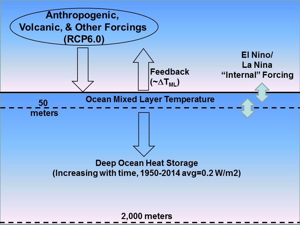
What is necessary is to have non-radiative forced variations in global-average surface temperature sufficiently large that they partly overcome the noise in the data. The largest single source of this non-radiative forcing is El Nino/La Nina, which correspond to a global-average weakening/strengthening of the overturning of the ocean.

It turns out that beating down noise (both measurement and geophysical) can be accomplished somewhat with time-averaging, so 3-monthly to annual averages can be used….whatever leads to the highest correlations.

Also, a time lag of 1 to 4 months is usually necessary because most of the net radiative feedback comes from the atmospheric response to a surface temperature change, which takes time to develop. Again, the optimum time lag is that which provides the highest correlation, and seems to be the longest (up to 4 months) with El Nino and La Nina events.

Anyway, here is the result for 15 years of annual CERES net radiative flux variations and HadCRUT4 surface temperature variations, with the radiative flux lagged 4 months after temperature:

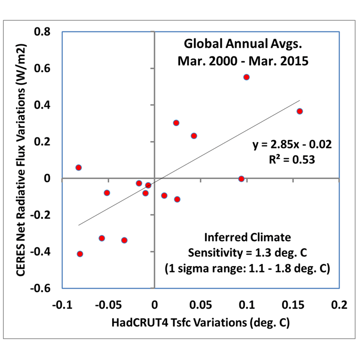
Fig. 1. Global, annual area averages of CERES-measured Net radiative flux variations against surface temperature variations from HadCRUT4, with a 4 month time lag to maximize correlation (flux after temperature).

Coincidentally, the 1.3 deg. C best estimate for the climate sensitivity from this graph is the same as we got with our 1D forcing-feedback-mixing climate model, and as I recently got with a simplified model that stores energy in the deep ocean at the observed rate (0.2 W/m2 average since the 1950s).

Again, the remaining radiative forcing in the 15 years of data causes decorrelation and (almost always) an underestimate of the feedback parameter (and overestimate of climate sensitivity). So, the real sensitivity might be well below 1.3 deg. C, as Lindzen believes. The inherent problem in diagnosing feedbacks from observational data is one which I am absolutely sure exists — and it is one which is largely ignored. Most of the “experts” who are part of the scientific consensus aren’t even aware of it, which shows how a small obscure issue can change our perception of how sensitive the climate system is.

This is also just one example of why hundreds (or even thousands) of “experts” agreeing on something as complex as climate change really doesn’t mean anything. It’s just group think in an echo chamber riding on a bandwagon.

Now, one can legitimately argue that the relationship in the above graph is still noisy, and so remains uncertain. But this is the most important piece of information we have to observationally determine how the real climate system responds radiatively to surface temperature changes, which then determines how big a problem global warming might be.

It’s clear that the climate models can be programmed to get just about any climate sensitivity one wants…currently covering a range of about a factor of 3! So, at some point we need to listen to what Mother Nature is telling us. And the above graph tells us that the climate system appears to be more stable than the experts believe.

Amid all of the debate over whether the global warming pause/hiatus exists or not, I’d like to bring people back to a central issue:

Even if it has warmed in the last 15 years, the rate of surface warming (and deep-ocean warming) we have seen in the last 50 years still implies low climate sensitivity.

I will demonstrate this with a simplified version of our 1D time-dependent energy balance model (Spencer & Braswell, 2014).

The reason why you can model global average climate system temperature variations with a simple energy balance model is that, given a certain amount of total energy accumulation or loss (in Joules) over the surface of the Earth in a certain amount of time, there will be a certain amount of warming or cooling of the depth-averaged ocean temperature. This is just a statement of energy conservation, and is non-controversial.

The rate of heat accumulation is the net of “forcing” and “feedback”, the latter of which stabilizes the climate system against runaway temperature change (yes, even on Venus). On multi-decadal time scales, we can assume without great error that the ocean is the dominant “heat accumulator” in climate change, with the land tagging along for the ride (albeit with a somewhat larger change in temperature, due to its lower effective heat capacity). The rate at which extra energy is being stored in the deep ocean has a large impact on the resulting surface temperature response.

The model feedback parameter lambda (which determines equilibrium climate sensitivity, ECS=3.8/lambda) is adjustable, and encompasses every atmospheric and surface process that changes in response to warming to affect the net loss of solar and infrared energy to outer space. (Every IPCC climate model will also have an effective lambda value, but it is the result of the myriad processes operating in the model, rather than simply specified).

Conceptually, the model looks like this:

Fig. 1. Simple time-dependent 1 layer model of global oceanic average mixed layer tamperature.

I have simplified the model so that, rather than having many ocean layers over which heat is diffused (as in Spencer & Braswell, 2014), there is just a top (mixed) layer that “pumps” heat downward at a rate that matches the observed increase in deep-ocean heat content over the last 50 years. This has been estimated to be 0.2 W/m2 since the 1950s increasing to maybe 0.5 W/m2 in the last 10 years.

I don’t want to argue whether this deep ocean warming might not even be occurring. Nor do I want to argue whether the IPCC-assumed climate forcings are largely correct. Instead, I want to demonstrate that , even if we assume these things AND assume the new pause-busting Karlized ocean surface temperature dataset is correct, it still implies low climate sensitivity.

Testing the Model Against CMIP5

If I run the model (available in spreadsheet form here) with the same radiative forcings used by the big fancy CMIP5 models (RCP 6.0 radiative forcing scenario), I get a temperature increase that roughly matches the average of all of the CMIP5 models, for the 60N-60S ocean areas (average CMIP5 results for the global oceans from the KNMI Climate Explorer):

Fig. 2. Simple model run to match the average of all CMIP5 models under the RCP 6.0 radiative forcing scenario.

The climate sensitivity I used to get this result was just over 2.5 C for a doubling of atmospheric CO2, which is consistent with published numbers for the typical climate sensitivity of many of these models. To be consistent with the CMIP5 models, I assume in 1950 that the climate system is 0.25 C warmer than the “normal balanced climate” state. This affects the model feedback calculation (the warmer the climate is assumed to be from “normal” the greater the loss of radiant energy to space). Of course, we really don’t know what the “normal balanced” state of the real climate system is…or even if there is one.

Running the Model to Match the New Pause-Busting Temperature Dataset

Now, let’s see how we have to change the climate sensitivity to match the new Karlized ERSST v4 dataset, which reportedly did away with the global warming pause:

Fig. 3. Simple model match to new pause-busting ERSST (v4) dataset.

In this case, we see that a climate sensitivity of only 1.5 C was required, a 40% reduction in climate sensitivity. Notably, this is at the 1.5C lower limit for ECS that the IPCC claims. Thus, even in the new pause-busting dataset the warming is so weak that it implies a climate sensitivity on the verge of what the IPCC considers “very unlikely”.

Running the Model to Match the New Pause-Busting Temperature Dataset (with ENSO internal forcing)

Finally, let’s look at what happens when we put in the observed history El Nino and La Nina events as a small radiative forcing (more incoming during El Nino, outgoing during La Nina, evidence for which was presented by Spencer & Braswell, 2014) and temporary internal energy exchanges between the mixed layer and deeper layers:

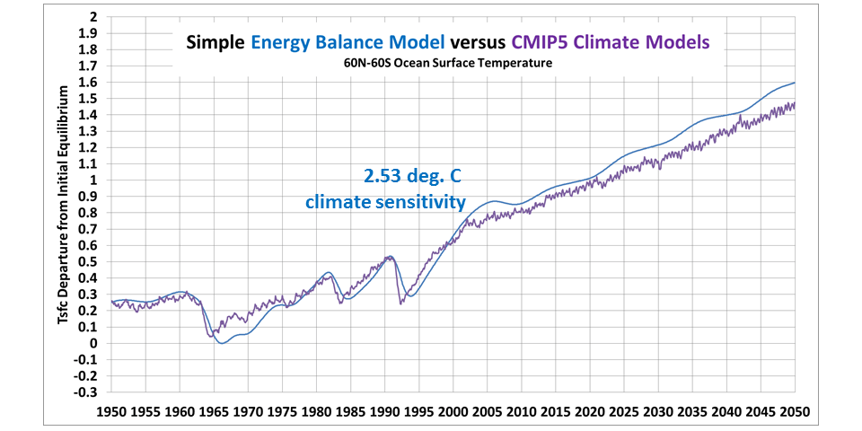
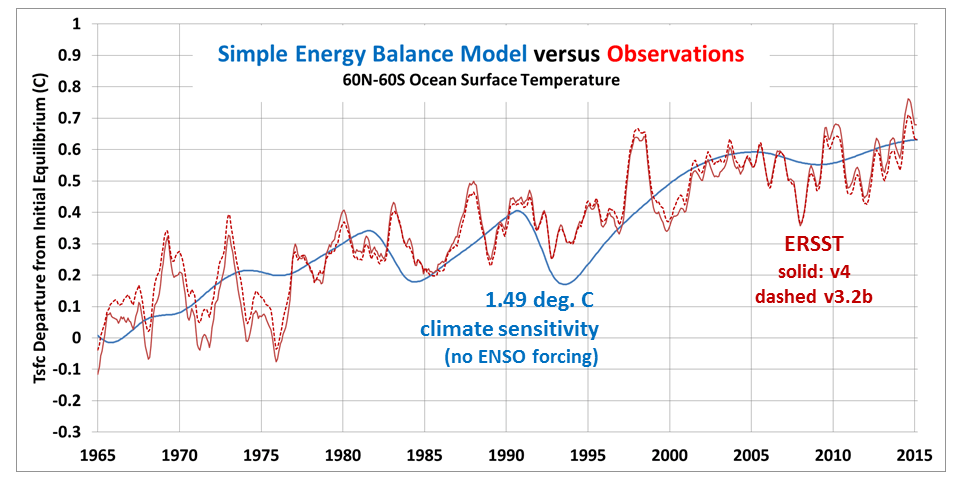
Fig. 4. As in Fig. 3, but with El Nino and La Nina variations included in the model (0.3 W/m2 per MEI unit radiative forcing, 0.4 W/m2 per MEI unit non-radiative forcing [heat excahnge between mixed layer and deeper layers]).

Now we have reduced the required climate sensitivity necessary to explain the observations to only 1.3 C, which is nearly a 50% ECS reduction below the 2.5C necessary to match the CMIP5 models. This result is similar to the one achieved by Spencer & Braswell (2014).

Comments

The simplicity of the model is not a weakness, as is sometimes alleged by our detractors — it’s actually a strength. Since the simple model time step is monthly, it avoids the potential for “energy leakage” in the numerical finite difference schemes used in big models during long integrations. Great model complexity does not necessarily get you closer to the truth.

In fact, we’ve had 30 years and billions of dollars invested in a marching army of climate modelers, and yet we are no closer to tying down climate sensitivity and thus estimates of future global warming and associated climate change. The latest IPCC report (AR5) gives a range from 1.5 to 4.5 C for a doubling of CO2, not much different from what it was 30 years ago.

There should be other simple climate model investigations like what I have presented above, where basic energy balance considerations combined with specific assumptions (like the deep oceans storing heat at an average rate of 0.2 W/m2 over the last 50 years) are used to diagnose climate sensitivity by matching the model to observations.

The IPCC apparently doesn’t do this, and I consider it a travesty that they don’t. 😉

I’ll leave it up to the reader to wonder why they don’t.

We discovered there were several days during June when communication problems prevented the transfer of some of the raw satellite data to our computer. This is an update of the June 2015 numbers with the missing satellite data included.

The Version 6.0 global average lower tropospheric temperature (LT) anomaly for June, 2015 is +0.33 deg. C, up somewhat from the May, 2015 value of +0.27 deg. C (click for full size version):

The global, hemispheric, and tropical LT anomalies from the 30-year (1981-2010) average for the last 6 months are:

YR MO GLOBE NH SH TROPICS
2015 1 +0.26 +0.38 +0.14 +0.12
2015 2 +0.16 +0.26 +0.05 -0.07
2015 3 +0.14 +0.23 +0.05 +0.02
2015 4 +0.06 +0.15 -0.02 +0.07
2015 5 +0.27 +0.33 +0.21 +0.27
2015 6 +0.33 +0.40 +0.26 +0.46

Notice the strong warming in the tropics over the last 2 months, consistent with the strengthening El Nino in the Pacific.

The global image for June, 2015 should be available in the next several days here.

The new Version 6 files, which should be updated soon, are located here:

Lower Troposphere: http://vortex.nsstc.uah.edu/data/msu/v6.0beta/tlt
Mid-Troposphere: http://vortex.nsstc.uah.edu/data/msu/v6.0beta/tmt
Tropopause: http://vortex.nsstc.uah.edu/data/msu/v6.0beta/ttp
Lower Stratosphere: http://vortex.nsstc.uah.edu/data/msu/v6.0beta/tls

Caution: For those who think I should stick to science, turn your eyes away now.

When my daughter studied in Greece several year ago, one of the first things she told me when she got there (and easily the most memorable) was “Dad, these people don’t know how to make money”.

Greeks, along with so many others in the world, have been fooled by the notion that prosperity can be achieved with a minimum of work. By “work” I mean as many people as possible, doing useful things for each other, as efficiently as possible.

No monetary policy or economic stimulus can supplant this basic truth. It is a necessary, but possibly not sufficient, requirement for prosperity. The role of government in this fundamentally private sector-driven process is to make sure people play fair, and then get out of the way.

When government bureaucrats become the ones who decide which goods and services are the most important, or what those should cost, or just how much of that wealth they will siphon off to give to those who don’t work, prosperity for a nation as a whole suffers.

I’ve long wondered how people can be fooled into believing work can be avoided, and the most central misconception I keep coming back to is this: If a person believes the same amount of stuff is going to be made anyway, then the only argument left is who gets how much, and the goal of an equitable distribution of wealth becomes central.

But one only need look around the world to see that wealth generation varies widely. It’s not even related to how many natural resources a country has, otherwise Japan would never have prospered and Russia should be one of the most prosperous countries on Earth. Haiti would be just as prosperous as Hong Kong.

The “constant pie” mindset was revealed by President Obama in his speech yesterday at the University of Wisconsin – La Crosse, when he said, “Being an American is not about taking as much as you can from your neighbor before they take as much as they can from you.”

Obama has mastered the art of presenting platitudes that sound on the surface like he’s a free market guy, but his policies end up not encouraging the generation of wealth, but instead redistributing wealth from the dwindling few who still generate it.

Since we do not teach basic economics to our children, this kind of message becomes seductive to the masses. It is an old message, historically, and it always ends badly.

There is no easy way to prosperity, just as there is no free lunch.

A second point often missing from the discussion is this: prosperity depends upon efficiency (e.g. mass production), which generally requires large investments. So, unless those with the means to invest have some hope of being able to keep their profits (since most will fail, and lose their investment), the system will not work.

Those few who have gotten immensely wealthy, generally speaking, have kept only a tiny fraction of the extra wealth they have generated for the country as a whole. They did not unfairly take from the rest of society; society freely gave it to them in exchange for something we wanted (e.g. iPhones).

When we threaten to take away their reward for a (risky) job well done, the system collapses. Politicians who then play the class envy card may gain some short term political points, but it will be at the expense of the country’s economic health.

In the 2015 Index of Economic Freedom, Heritage Foundation ranks Greece 130th out of 178 countries (Venezuela, Cuba, and North Korea rank last). Yet, this Forbes article with opinions from 3 Harvard Business School professors asked to comment on the Greek crisis fails to even bring up this systemic problem, and instead offers only vague platitudes.

So, again, any government economic policy must (in my admittedly simple minded opinion) always be judged against the single overriding goal for a country hoping to achieve prosperity: “As many people as possible, doing useful things for each other, as efficiently as possible.”

If a government’s policies cannot support that basic goal, there will be nothing of value to govern, and the original poor among us (whose numbers will increase dramatically) will be even worse off than they were before.

Now back to our regularly scheduled programming.

NOTE: This is the third monthly update with our new Version 6.0 dataset. Differences versus the old Version 5.6 dataset are discussed here.

The Version 6.0 global average lower tropospheric temperature (LT) anomaly for June, 2015 is +0.31 deg. C, up a little from the May, 2015 value of +0.27 deg. C (click for full size version):

The global, hemispheric, and tropical LT anomalies from the 30-year (1981-2010) average for the last 6 months are:

YR MO GLOBE NH SH TROPICS
2015 1 +0.26 +0.38 +0.14 +0.12
2015 2 +0.16 +0.26 +0.05 -0.07
2015 3 +0.14 +0.23 +0.05 +0.02
2015 4 +0.06 +0.15 -0.02 +0.07
2015 5 +0.27 +0.33 +0.21 +0.27
2015 6 +0.31 +0.36 +0.26 +0.46

Notice the strong warming in the tropics over the last 2 months, consistent with the strengthening El Nino in the Pacific.

The global image for June, 2015 should be available in the next several days here.

The new Version 6 files, which should be updated soon, are located here:

Lower Troposphere: http://vortex.nsstc.uah.edu/data/msu/v6.0beta/tlt
Mid-Troposphere: http://vortex.nsstc.uah.edu/data/msu/v6.0beta/tmt
Tropopause: http://vortex.nsstc.uah.edu/data/msu/v6.0beta/ttp
Lower Stratosphere: http://vortex.nsstc.uah.edu/data/msu/v6.0beta/tls