Archive for November, 2020

Benford’s Law, Part 2: Inflated Vote Totals, or Just the Nature of Precinct Sizes?

Thursday, November 12th, 2020

SUMMARY: Examination of vote totals across ~6,000 Florida precincts during the 2016 presidential election shows that a 1st digit Benford’s type analysis can seem to suggest fraud when precinct vote totals have both normal and log-normal distribution components. Without prior knowledge of what the precinct-level vote total frequency distribution would be in the absence of fraud, I see no way to apply 1st digit Benford’s Law analysis to deduce fraud. Any similar analysis would have the same problem, because it depends upon the expected frequency distribution of vote totals, which is difficult to estimate because it is tantamount to knowing a vote outcome absent fraud. Instead, it might be more useful to simply examine the precinct-level vote distributions, rather than Benford-type analysis of those data, and compare one candidate’s distribution to that of other candidates.

It has been only one week since someone introduced me to Benford’s Law as a possible way to identify fraud in elections. The method looks at the first digit of all vote totals reported across many (say, thousands) of precincts. If the vote totals in the absence of fraudulently inflated values can be assumed to have either a log-normal distribution or a 1/X distribution, then the relative frequency of the 1st digits (1 through 9) have very specific values, deviations from which might suggest fraud.

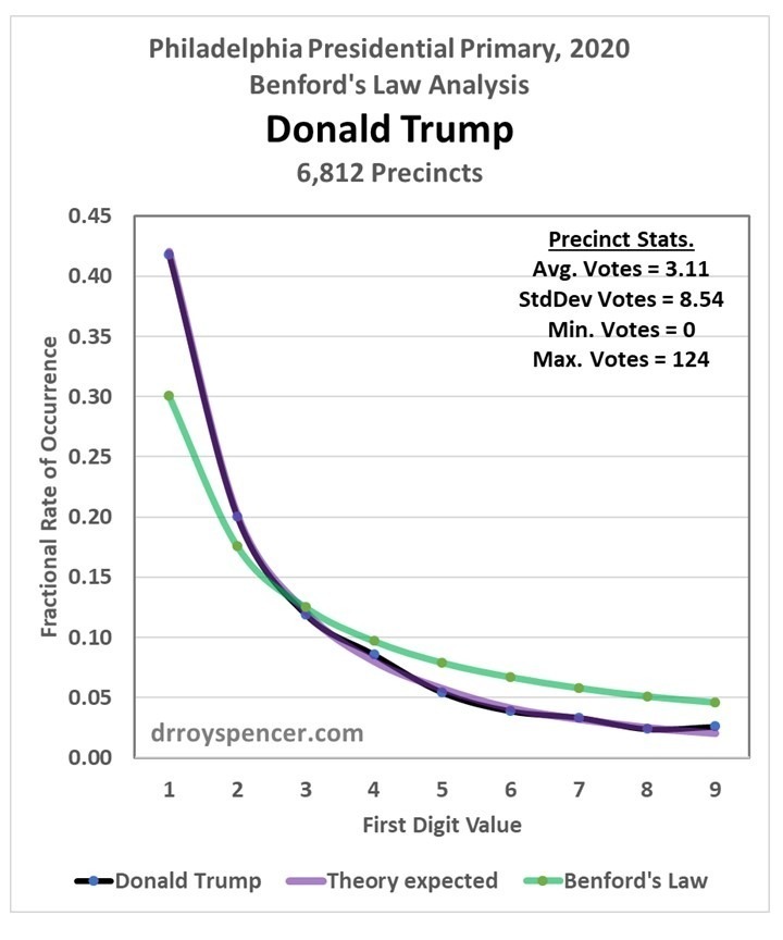
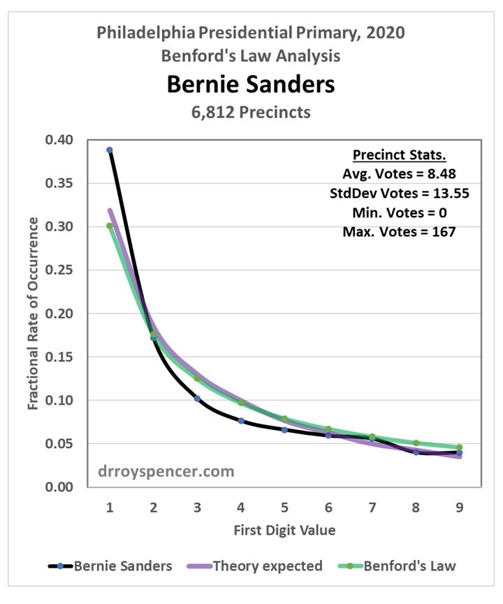
After a weekend examining vote totals from Philadelphia during the 2020 presidential primary, my results were mixed. Next, I decided to examine Florida precinct level data from the 2016 election (data from the 2020 general election are difficult to find). My intent was to determine whether Benford’s Law can really be applied to vote totals when there was no evidence of widespread fraud. In the case of Trump votes in the 2020 primary in Philadelphia, the answer was yes, the data closely followed Benford. But that was just one election, one candidate, and one city.

When I analyzed the Florida 2016 general election data, I saw departures from Benford’s Law in both Trump and Clinton vote totals:

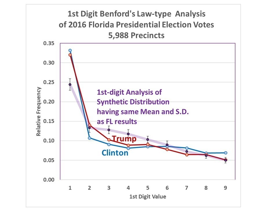
Fig. 1. First-digit Benford’s Law-type analysis of 2016 presidential vote totals for Trump and Clinton in Florida, compared to that of a synthetic log-normal distribution having the same mean and standard deviations as the actual vote data, with 99% confidence level of 100 log-normal distributions with the same sample size.

For at least the “3” and “4” first digit values, the results are far outside what would be expected if the underlying vote frequency distribution really was log-normal.

This caused me to examine the original frequency distributions of the votes, and then I saw the reason why: Both the Trump and Clinton frequency distributions exhibit elements of both log-normal and normal distribution shapes.

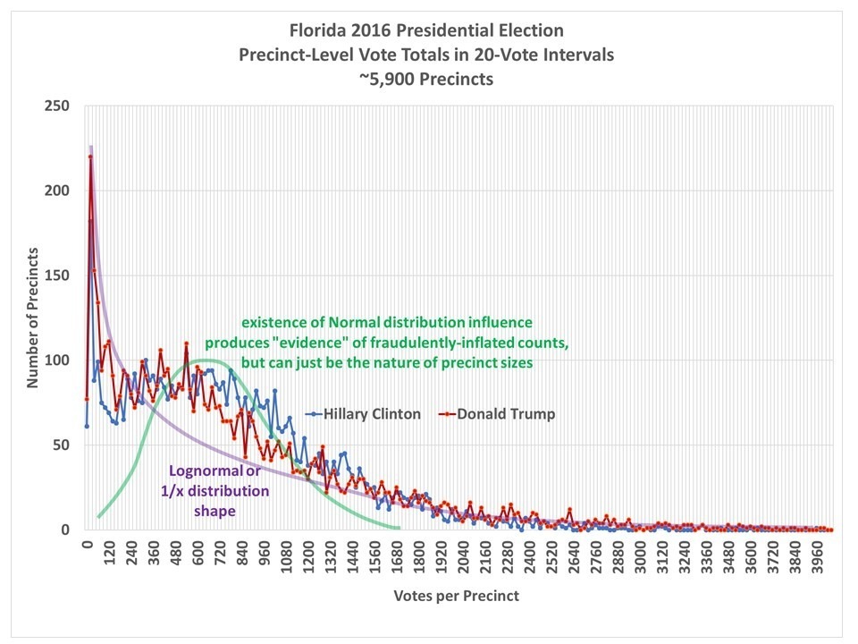
Fig. 2. Frequency distributions of the precinct-level vote totals in Florida during the 2016 general election. Both Trump and Clinton distributions show evidence of log-normal and normal distribution behavior. Benford’s Law analysis only applies to log-normal (or 1/x) distributions.

And this is contrary to the basis for Bendford’s Law-type analysis of voting data: It assumes that vote totals follow a specific frequency distribution (lognormal or 1/x), and if votes are fraudulently added (AND those fake additions are approximately normally distributed!), then the 1st-digit analysis will depart from Benford’s Law.

Since Benford’s Law analysis depends upon the underlying distribution being pure lognormal (or 1/x power law shape), it seems that understanding the results of any Benford’s Law analysis depends upon the expected shape of these voting distributions… and that is not a simple task. Is the expected distribution of vote totals really log-normal?

Why Should Precinct Vote Distributions have a Log-normal Shape?

Benford’s Law analyses of voting data depend upon the expectation that there will be many more precincts with low numbers of votes cast than precincts with high numbers of votes. Voting locations in rural areas and small towns will obviously not have as many voters as do polling places in large cities, and presumably there will be more of them.

As a result, precinct-level vote totals will tend to have a frequency distribution with more low-vote totals, and fewer high vote totals. In order to produce Benford’s Law type results, the distribution must have either a log-normal or a power law (1/x) shape.

But there are reasons why we might expect vote totals to also exhibit more of a normal-type (rather than log-normal) distribution.

Why Might Precinct-Level Vote Totals Depart from Log-Normal?

While I don’t know the details, I would expect that the number of voting locations would be scaled in such a way that each location can handle a reasonable level of voter traffic, right?

For the sake of illustration of my point, one might imagine a system where ALL voting locations, whether urban or rural, were optimally designed to handle roughly 1,000 voters at expected levels of voter turnout.

In the cities maybe these would be located every few blocks. In rural Montana, some voters might have to travel 100 miles to vote.   In this imaginary system, I think you can see that the precinct-level vote totals would then be more normally distributed, with an average of around 1,000 votes and just as many 500-vote precincts as 1,500 vote precincts (instead of far more low-vote precincts than high-vote precincts, as is currently the case).

But, we wouldn’t want rural voters to have to drive 100 miles to vote, right? And there might not be enough public space to have voting locations every 2 blocks in a city, and as a results some VERY high vote totals can be expected from crowded urban voting locations.

So, we instead have a combination of the two distributions: log-normal (because there are many rural locations with few voters, and some urban voting places that are over-crowded) and normal (because cities will tend to have precinct locations optimized to handle a certain number of voters, as best they can).

Benford-Type Analysis of Synthetic Normal and Log-normal Distributions

If I create two sets of synthetic data, 100,000 values in each, one with a normal distribution and one with a log-normal distribution, this is what the relative frequencies of the 1st digit of those vote totals looks like:

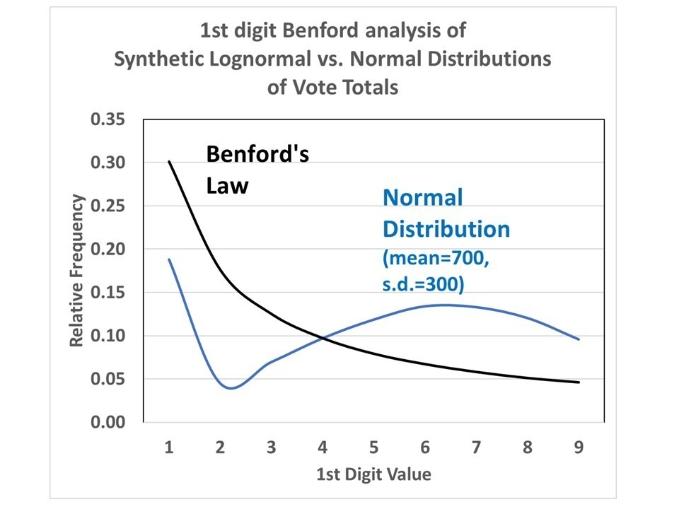
Fig. 3. 1st-digit analysis of a normal frequency distribution versus a long-normal distribution (Benford’s Law).

The results for a normal distribution move around quite a lot, depending upon the assumed mean and standard deviation of that distribution.

I believe that what is going on in the Florida precinct data is simply a combination of normal and log-normal distributions of the vote totals. So, for a variety of reasons, the vote totals do not follow a log-normal distribution and so cannot be interpreted with Benford’s Law-type analyses.

One can easily imagine other reasons for the frequency distribution of precinct-level votes to depart from log-normal.

What one would need is convincing evidence of that the frequency distribution should look like in the absence of fraud. But I don’t see how that is possible, unless one candidate’s vote distribution is extremely skewed relative to another candidate’s vote totals, or compared to primary voting totals.

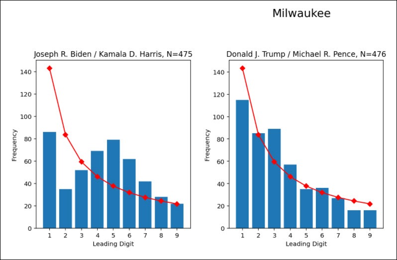
And this is what happened in Milwaukee (and other cities) in the most recent elections: The Benford Law analysis suggested very different frequency distributions for Trump than for Biden.

I would think it is more useful to just look at the raw precinct-level vote distributions (e.g. like Fig. 2) rather than a Benford analysis of those data. The Benford analysis technique suggests some sort of magical, universal relationship, but it is simply the result of a log-normal distribution of the data. Any departure from the Benford percentages is simply a reflection of the underlying frequency distribution departing from log-normal, and not necessarily indicative of fraud.

Benford’s Law: Evidence of Fraud in Reporting of Voter Precinct Totals?

Monday, November 9th, 2020

You might have seen reports in the last several days regarding evidence of fraud in ballot totals reported in the presidential election. There is a statistical relationship known as “Benford’s Law” which states that for many real-world distributions of numbers, the frequency distribution of the first digit of those numbers follows a regular pattern. It has been used by the IRS and financial institutions to detect fraud.

It should be emphasized that such statistical analysis cannot prove fraud. But given careful analysis including the probability of getting results substantially different from what is theoretically-expected, I think it is a useful tool. Its utility is especially increased if there is little or no evidence of fraud for one candidate, but strong evidence of fraud from another candidate, across multiple cities or multiple states.

From Wikipedia:

“Benford’s law, also called the Newcomb-Benford law, the law of anomalous numbers, or the first-digit law, is an observation about the frequency distribution of leading digits in many real-life sets of numerical data. The law states that in many naturally occurring collections of numbers, the leading digit is likely to be small. For example, in sets that obey the law, the number 1 appears as the leading significant digit about 30% of the time, while 9 appears as the leading significant digit less than 5% of the time. If the digits were distributed uniformly, they would each occur about 11.1% of the time. Benford’s law also makes predictions about the distribution of second digits, third digits, digit combinations, and so on.”

For example, here’s one widely circulating plot (from Github) of results from Milwaukee’s precincts, showing the Benford-type plots for Trump versus Biden vote totals.

Fig. 1. Benford-type analysis of Milwaukee precinct voting data, showing a large departure of the voting data (blue bars) from the expected relationship (red line) for Biden votes, but agreement for the Trump votes. This is for 475 voting precincts. (This is not my analysis, and I do not have access to the underlying data to check it).

The departure from statistical expectations in the Biden vote counts is what is expected when some semi-arbitrary numbers, presumably small enough to not be easily noticed, are added to some of the precinct totals. (I verified this with simulations using 100,000 random but log-normally distributed numbers, where I then added 1,2,3, etc. votes to individual precinct totals). The frequency of low digit values are reduced, while the frequency of the higher digit values are raised.

Since I like the analysis of large amounts of data, I thought I would look into this issue with some voting data. Unfortunately, I cannot find any precinct-level data for the general election. So, I instead looked at some 2020 presidential primary data, since those are posted at state government websites. So far I have only looked at the data from Philadelphia, which has a LOT (6,812) of precincts (actually, “wards” and “divisions” within those wards). I did not follow the primary election results from Philadelphia, and I have no preconceived notions of what the results might look like; these were just the first data I found on the web.

Results for the Presidential Primary in Philadelphia

I analyzed the results for 4 candidates with the most primary votes in Philadelphia: Biden, Sanders, Trump, and Gabbard (data available here).

Benford’s Law only applies well to data that that covers at least 2-3 orders of magnitude (say, from 0 to in the hundreds or thousands). In the case of a candidate who received very few votes, an adjustment to Benford’s relationship is needed.

The most logical way to do this (for me) was to generate a synthetic set of 100,000 random, but log-normally distributed numbers ranging from zero and up, but adjusted until the mean and standard deviation of the data matched the voting data for each candidate separately. (The importance of using a log-normal distribution was suggested to me by a statistician, Mathew Crawford, who works in this area). Then, you can do the Benford analysis (frequency of the 1st digits of those numbers) to see what is theoretically-expected, and then compare to the actual voting data.

Donald Trump Results

First, let’s look at the analysis for Donald Trump during the 2020 presidential primary in Philadelphia (Fig. 2). Note that the Trump votes agree very well with the theoretically-expected frequencies (purple line). The classical Benford Law values (green line) are quite different because the range of votes for Trump only went up to 124 votes, with an average of only 3.1 votes for Trump per precinct.

So, in the case of Donald Trump primary votes in Philadelphia, the results are extremely close to what is expected for log-normally distributed vote totals.

Fig. 2. Benford-type analysis of the number of Trump votes across 6,812 Philadelphia precincts. The classical Benford Law expected distribution of the 1st digits in the vote total is in green. The adjusted Benford Law results based upon 100,000 random but log-normally distributed vote values having the same mean and standard deviation as the vote data in in purple. The actual results from the vote data are in black.

Tulsi Gabbard Results

Next, let’s look at what happens when even fewer votes are cast for a candidate, in this case Tulsi Gabbard (Fig. 3). In this case the number of votes was so small that I could not even get the synthetic log-normal distribution to match the observed precinct mean (0.65 votes) and standard deviation (1.29 votes). So, I do not have high confidence that the purple line is a good expectation of the Gabbard results. (This, of course, will not be a problem with major candidates).

Fig. 3. As in Fig. 2, but for Tulsi Gabbard.

Joe Biden Results

The results for Joe Biden in the Philadelphia primary vote show some evidence for a departure of the reported votes (black line) from theory (purple line) in the direction of inflated votes, but I would need to launch into an analysis of the confidence limits; it could be the observed departure is within what is expected given random variations in this number of data (N=6,812).

Fig. 4. As in Fig. 2, but for Joe Biden.

Bernie Sanders Results

The most interesting results are for Bernie Sanders (Fig. 5.), where we see the largest departure of the voting data (black line) from theoretical expectations (purple line). But instead of reduced frequency of low digits, and increased frequency of higher digits, we see just the opposite.

Is this evidence of fraud in the form of votes subtracted from Sanders’ totals? I don’t know… I’m just presenting the results.

Fig. 5. As in Fig 2, but for Bernie Sanders.

Conclusions

It appears that a Benford’s Law- type of analysis would be useful for finding evidence of fraudulently inflated (or maybe reduced?) voter totals. Careful confidence level calculations would need to be performed, however, so one could say whether the departures from what is theoretically expected are larger than, say, 95% or 99% of what would be expected from just random variations in the reported totals.

I must emphasize that my conclusions are based upon analysis of these data over only a single weekend. There are people who do this stuff for a living. I’d be glad to be corrected on any points I have made. Part of my reason for this post is to introduce people to what is involved in these calculations, after understanding it myself, since it is now part of the public debate over the 2020 presidential election results.

UAH Global Temperature Update for October 2020: +0.54 deg. C

Monday, November 2nd, 2020

The Version 6.0 global average lower tropospheric temperature (LT) anomaly for October, 2020 was +0.54 deg. C, down slightly from the September, 2020 value of +0.57 deg. C.

The linear warming trend since January, 1979 remains at +0.14 C/decade (+0.12 C/decade over the global-averaged oceans, and +0.18 C/decade over global-averaged land).

For comparison, the CDAS global surface temperature anomaly for the last 30 days at Weatherbell.com was +0.33 deg. C.

With La Nina in the Pacific now officially started, it will take several months for that surface cooling to be fully realized in the tropospheric temperatures. Typically, La Nina minimum temperatures (and El Nino maximum temperatures) show up around February, March, or April.

Various regional LT departures from the 30-year (1981-2010) average for the last 22 months are:

YEAR MO GLOBE NHEM. SHEM. TROPIC USA48 ARCTIC AUST 
2019 01 +0.38 +0.35 +0.41 +0.36 +0.53 -0.14 +1.14
2019 02 +0.37 +0.47 +0.28 +0.43 -0.02 +1.05 +0.05
2019 03 +0.34 +0.44 +0.25 +0.41 -0.55 +0.97 +0.58
2019 04 +0.44 +0.38 +0.51 +0.54 +0.49 +0.93 +0.91
2019 05 +0.32 +0.29 +0.35 +0.39 -0.61 +0.99 +0.38
2019 06 +0.47 +0.42 +0.52 +0.64 -0.64 +0.91 +0.35
2019 07 +0.38 +0.33 +0.44 +0.45 +0.10 +0.34 +0.87
2019 08 +0.39 +0.38 +0.39 +0.42 +0.17 +0.44 +0.23
2019 09 +0.61 +0.64 +0.59 +0.60 +1.14 +0.75 +0.57
2019 10 +0.46 +0.64 +0.27 +0.30 -0.03 +1.00 +0.49
2019 11 +0.55 +0.56 +0.54 +0.55 +0.21 +0.56 +0.37
2019 12 +0.56 +0.61 +0.50 +0.58 +0.92 +0.66 +0.94
2020 01 +0.56 +0.60 +0.53 +0.61 +0.73 +0.13 +0.65
2020 02 +0.76 +0.96 +0.55 +0.76 +0.38 +0.02 +0.30
2020 03 +0.48 +0.61 +0.34 +0.63 +1.09 -0.72 +0.16
2020 04 +0.38 +0.43 +0.33 +0.45 -0.59 +1.03 +0.97
2020 05 +0.54 +0.60 +0.49 +0.66 +0.17 +1.16 -0.15
2020 06 +0.43 +0.45 +0.41 +0.46 +0.38 +0.80 +1.20
2020 07 +0.44 +0.45 +0.42 +0.46 +0.56 +0.40 +0.66
2020 08 +0.43 +0.47 +0.38 +0.59 +0.41 +0.47 +0.49
2020 09 +0.57 +0.58 +0.56 +0.46 +0.97 +0.48 +0.92
2020 10 +0.54 +0.71 +0.37 +0.37 +1.10 +1.23 +0.24

The full UAH Global Temperature Report, along with the LT global gridpoint anomaly image for October, 2020 should be available within the next few days here.

The global and regional monthly anomalies for the various atmospheric layers we monitor should be available in the next few days at the following locations:

Lower Troposphere: http://vortex.nsstc.uah.edu/data/msu/v6.0/tlt/uahncdc_lt_6.0.txt
Mid-Troposphere: http://vortex.nsstc.uah.edu/data/msu/v6.0/tmt/uahncdc_mt_6.0.txt
Tropopause: http://vortex.nsstc.uah.edu/data/msu/v6.0/ttp/uahncdc_tp_6.0.txt
Lower Stratosphere: http://vortex.nsstc.uah.edu/data/msu/v6.0/tls/uahncdc_ls_6.0.txt