Home/Blog
As part of a DOE contract John Christy and I have, we are using satellite data to examine climate model behavior. One of the problems I’ve been interested in is the effect of El Nino and La Nina (ENSO) on our understanding of human-caused climate change. A variety of ENSO records show multi-decadal variations in this activity, and it has even showed up in multi-millennial runs of a GFDL climate model.
Since El Nino produces global average warmth, and La Nina produces global average coolness, I have been using our 1D forcing feedback model of ocean temperatures (published by Spencer & Braswell, 2014) to examine how the historical record of ENSO variations can be included, by using the CERES satellite-observed co-variations of top-of-atmosphere (TOA) radiative flux with ENSO.
I’ve updated that model to match the 20 years of CERES data (March 2000-March 2020). I have also extended the ENSO record back to 1525 with the Braganza et al. (2009) multi-proxy ENSO reconstruction data. I intercalibrated it with the Multivariate ENSO Index (MEI) data up though the present, and further extended into mid-2021 based upon the latest NOAA ENSO forecast. The Cheng et al. temperature data reconstruction for the 0-2000m layer is also used to calibrate the model adjustable coefficients.
I had been working on an extensive blog post with all of the details of how the model works and how ENSO is represented in it, which was far too detailed. So, I am instead going to just show you some results, after a brief model description.
1D Forcing-Feedback Model Description
The model assumes an initial state of energy equilibrium, and computes the temperature response to changes in radiative equilibrium of the global ocean-atmosphere system using the CMIP5 global radiative forcings (since 1765), along with our calculations of ENSO-related forcings. The model time step is 1 month.
The model has a mixed layer of adjustable depth (50 m gave optimum model behavior compared to observations), a second layer extending to 2,000m depth, and a third layer extending to the global-average ocean bottom depth of 3,688 m. Energy is transferred between ocean layers proportional to their difference in departures from equilibrium (zero temperature anomaly). The proportionality constant(s) have the same units as climate feedback parameters (W m-2 K-1), and are analogous to the heat transfer coefficient. A transfer coefficient of 0.2 W m-2 K-1 for the bottom layer produced 0.01 deg. C of net deep ocean warming (below 2000m) over the last several decades which Cheng et al. mentioned there is some limited evidence for.
The ENSO related forcings are both radiative (shortwave and longwave), as well as non-radiative (enhanced energy transferred from the mixed layer to deep ocean during La Nina, and the opposite during El Nino). These are discussed more in our 2014 paper. The appropriate coefficients are adjusted to get the best model match to CERES-observed behavior compared to the MEIv2 data (2000-2020), observed SST variations, and observed deep-ocean temperature variations. The full 500-year ENSO record is a combination of the Braganza et al. (2009) year data interpolated to monthly, the MEI-extended, MEI, and MEIv2 data, all intercalibrated. The Braganza ENSO record has a zero mean over its full period, 1525-1982.
Results
The following plot shows the 1D model-generated global average (60N-60S) mixed layer temperature variations after the model has been tuned to match the observed sea surface temperature temperature trend (1880-2020) and the 0-2000m deep-ocean temperature trend (Cheng et al., 2017 analysis data).
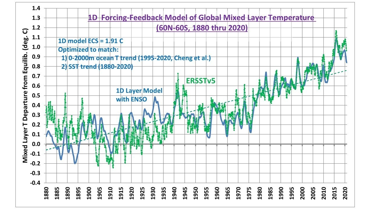
Fig. 1. 1D model temperature variations for the global oceans (60N-60S) to 50 m depth, compared to observations.
Note that the specified net radiative feedback parameter in the model corresponds to an equilibrium climate sensitivity of 1.91 deg. C. If the model was forced to match the SST observations during 1979-2020, the ECS was 2.3 deg. C. Variations from these values also occurred if I used HadSST1 or HadSST4 data to optimize the model parameters.
The ECS result also heavily depends upon the accuracy of the 0-2000 meter ocean temperature measurements, shown next.
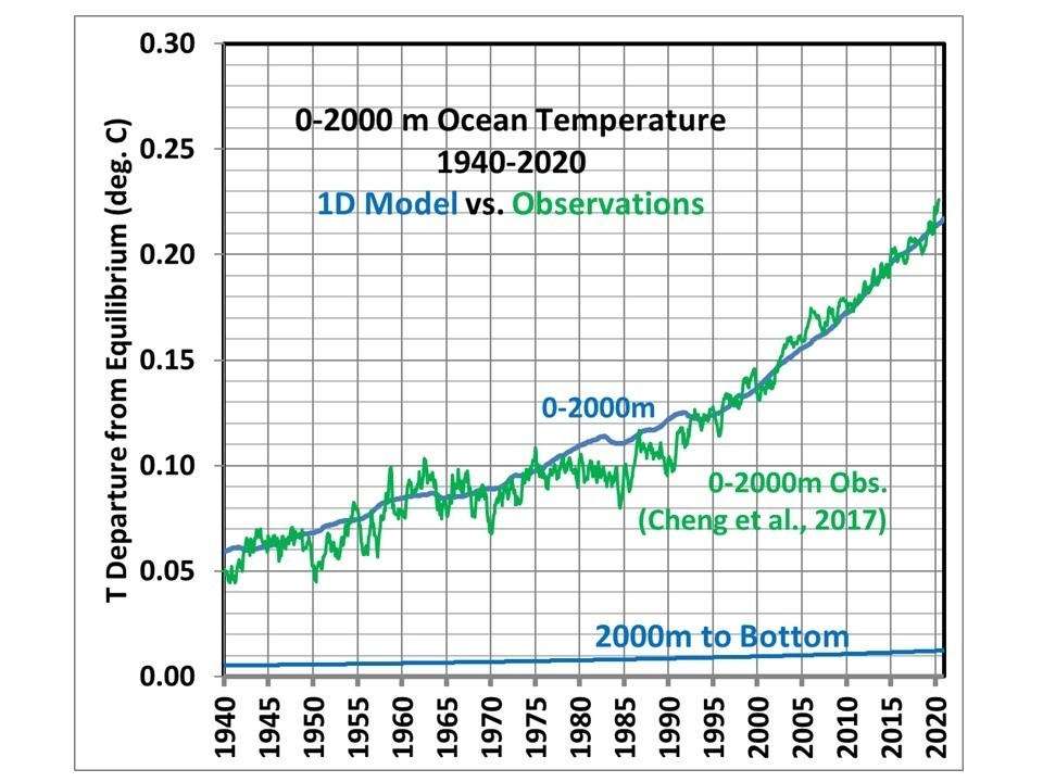
Fig. 2. 1D model temperature changes for the 0-2000m layer since 1940, and compared to observations.
The 1D model was optimized to match the 0-2000m temperature trend only since 1995, but we see in Fig. 2 that the limited data available back to 1940 also shows a reasonably good match.
Finally, here’s what the full 500 year model results look like. Again, the CMIP5 forcings begin only in 1765 (I assume zero before that), while the combined ENSO dataset begins in 1525.
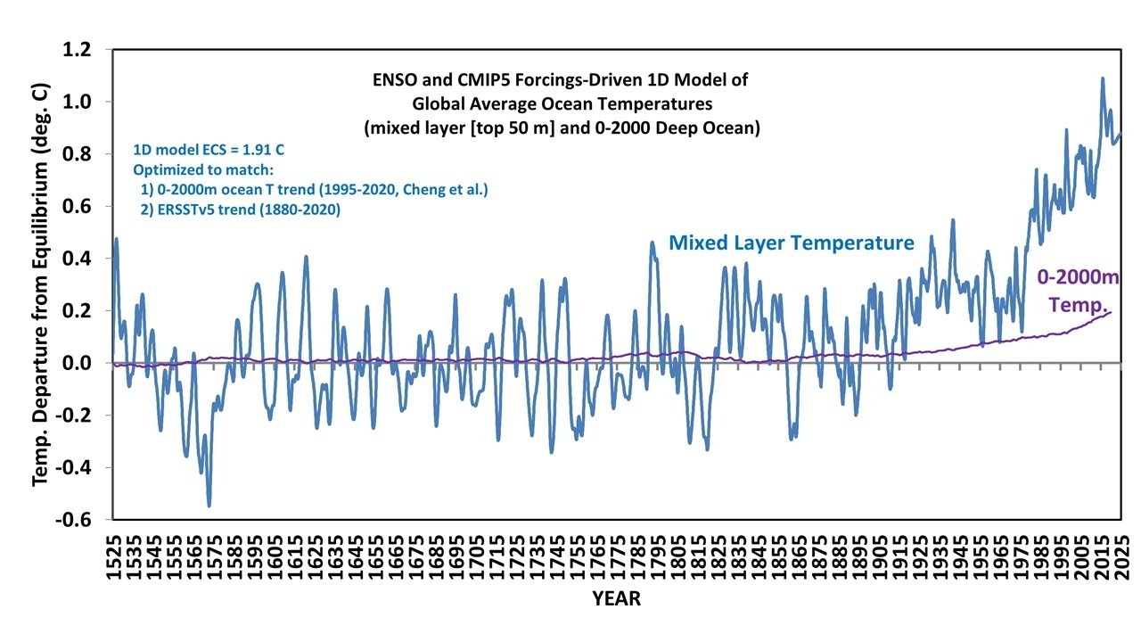
Fig. 3. Model results extended back to 1525 with the proxy ENSO forcings, and since 1765 with CMIP5 radiative forcings.
Discussion
The simple 1D model is meant to explain a variety of temperature-related observations with a physically-based model with only a small number of assumptions. All of those assumptions can be faulted in one way or another, of course.
But the monthly correlation of 0.93 between the model and observed SST variations, 1979-2020, is very good (0.94 for 1940-2020) for it being such a simple model. Again, our primary purpose was to examine how observed ENSO activity affects our interpretation of warming trends in terms of human causation.
For example, ENSO can then be turned off in the model to see how it affects our interpretation of (and causes of) temperature trends over various time periods. Or, one can examine the affect of assuming some level of non-equilibrium of the climate system at the model initialization time.
If nothing else, the results in Fig. 3 might give us some idea of the ENSO-related SST variations for 300-400 years before anthropogenic forcings became significant, and how those variations affected temperature trends on various time scales. For if those naturally-induced temperature trend variations existed before, then they still exist today.