As discussed over at WUWT, there has been a significant change in NOAA’s Climate Forecast System (CFSv2) model resulting from a cold bias that has been developing in the model in the tropical Atlantic ocean temperatures.

Since the NOAA presentation regarding the CFSv2 model problem made it sound like they haven’t been routinely adding ocean observations to the model, I asked NOAA’s David Behringer for clarification, and he said:

“First, to be clear, the ocean component of the CFSv2 is routinely updated with the thousands of ocean observations provided daily by many platforms (Argo drifters, TAO-TRITON and other tropical moorings, satellites, etc.) via a variational assimilation method.

At the root of the problem is what is sometimes referred to as the representation error: the mismatch between what the numerical ocean model can resolve versus what the set of ocean observations provide, which are very accurate point measurements of the real ocean. In effect, your reasoning was on the right track, but I would turn it around: it is the inherent limitations of the ocean model, not the accuracy of the observations, that ultimately caused this particular failure.

Let me say a little more about this specific case. The ocean model used in the CFSv2 is built on a variable grid; the resolution over most of the globe is1/2 degree, but within 10 degrees of the equator it is 1/4 degree. A 1/4-dgree grid is considered to be “eddy permitting”, but not “eddy resolving”, meaning that the model dynamics will generate eddies, but these eddies cannot be made to match up with real world eddies. In the 1/2-degree part of the grid we do a reasonably good job managing the representation error through the specification of model and observational error variances, but in the 1/4-degree equatorial zone the job is much harder. In the equatorial zone of the western Atlantic, which is very energetic, the job is harder yet.

The answer is a better assimilation system. The ocean 3D variational (3dvar) system used in the CFSv2 provides a global solution. So we can have a situation where the 3dvar believes the analysis has converged globally, but locally where model-observation differences are too large, for reasons described above, it may not have converged. I think this is what has happened in the CFSv2. We have made improvements to the 3dvar and it is working successfully offline. However, it will need further testing offline before it can be made operational. A temporary emergency fix will be used in the meantime.“

Now, I’m not a 3D modeler, but I think what he’s saying is that the numerics in the model in the tropical Atlantic generate unrealistic small-scale ocean eddies in this particularly energetic region that are too intense for the global real-data assimilation system to remove, and they have a temporary model fix in place. (For those not familiar, weather forecast models are typically initialized with a mixture of observations and a previous model forecast, called “3DVAR” methodology, since there is not enough observational data alone to describe the 3D state of the ocean-atmosphere system at any given time.)

Since I was still a little confused about whether the Atlantic cold spot would just reemerge in a many-month model forecast, I asked Dave for clarification on this. He responded:

“In this particular case the Atlantic cold spot was caused by a flaw in the data assimilation. Once that was corrected and the cold spot removed, it should not return during the forecast cycle.“

Ryan Maue at Weatherbell.com (which is well worth the $20/month subscription fee to get their full range of model output) provided me some imagery of how the La Nina forecast for later this year suddenly appeared in the CFSv2 model after the cold Atlantic fix was implemented:

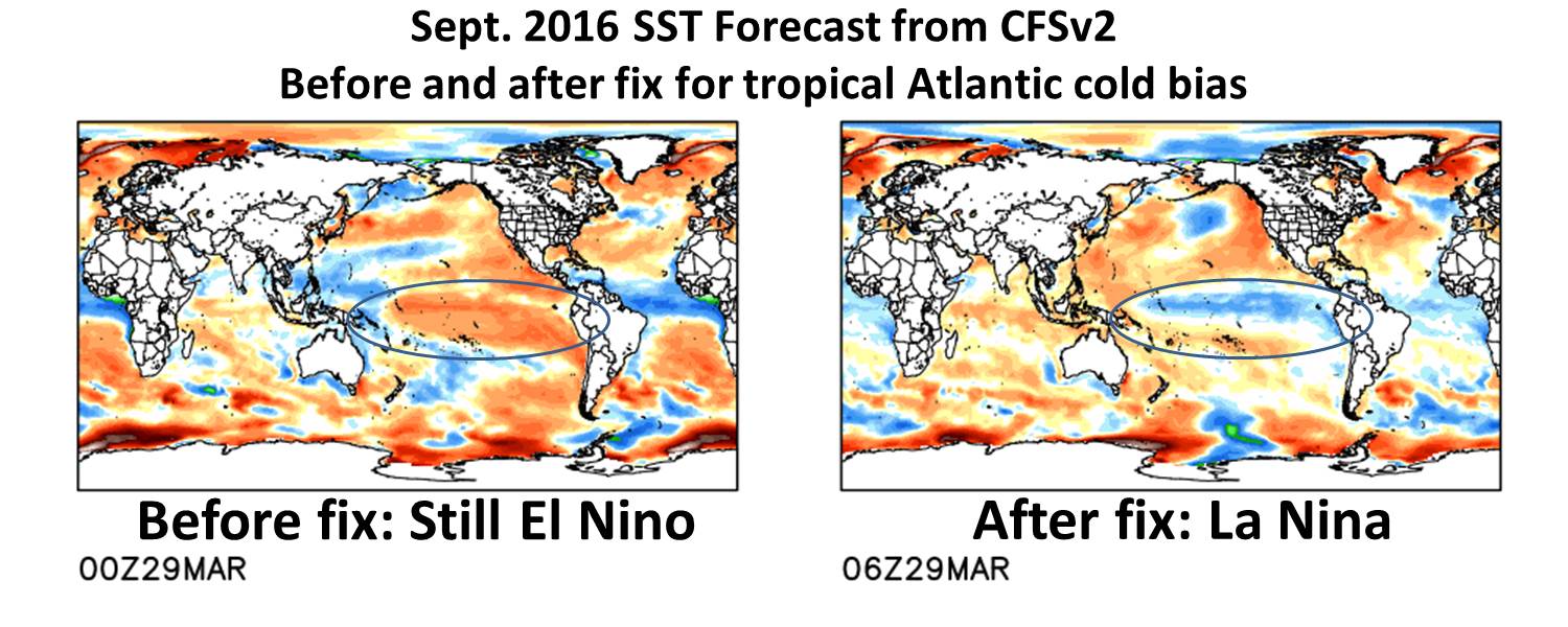
Sept. 2016 SST forecast from the CFSv2 model before and after a fix was made for anomalously cold water in the tropical Atlantic (courtesy Ryan Maue, Weatherbell.com).

This fix now puts the CFSv2 model forecast of La Nina more in line with the general cluster of ENSO forecasts, which suggest La Nina conditions by late summer or early fall.

The eruption of Pavlof volcano in Alaska’s Aleutian Islands late Sunday was sudden, and produced a massive brown ash cloud as seen in yesterday’s MODIS imagery from NASA’s Terra satellite (click for large version):

The Coast Guard took this photo from one of their aircraft at about the same time as the satellite overpass:

I suspect that it is unlikely that the ash cloud will have much effect on climate due to the relatively small size of the eruption, the high latitude of the volcano, and a probable lack of sulfur emissions into the stratosphere. Tropical stratovolcano eruptions have the biggest effect on climate since volcanic emissions reaching the tropical stratosphere tend to spread over most of the Earth.

A George Mason University survey of 4,092 members of the American Meteorological Society (AMS) on climate change attitudes in the meteorological community has just been released.

It shows fairly general acceptance of the view that climate change is happening, that it is at least partly due to humans, and that we can mitigate it somewhat by our energy policies.

Fully 37% of those surveyed (including me) consider themselves “expert” in climate science. It should be remembered that most of us old climate researchers were formally trained as meteorologists, with climatology being just a small part of our education.

But what I find interesting is that the supposed 97% consensus on climate change (which we know is bogus anyway) turns into only 67% when we consider the number of people who believe climate change is mostly or entirely caused by humans, as indicated by this bar chart:

George Mason University survey results of 4,092 members of the American Meteorological Society.

Fully 33% either believe climate change is not occurring, is mostly natural, or is at most half-natural and half-manmade (I tend toward that last category)…or simply think we “don’t know”.

For something that is supposed to be “settled science”, I find that rather remarkable.

The revelation that AG Loretta Lynch had discussions about bringing charges against climate change deniers (I’ve yet to meet a ‘climate change denier’) has led to a few questions about whether people like me (a skeptic of the view that the human influence on climate is either large or dangerous) should be worried.

What? Me worry?

Actually, I do tend to be a worrier. I’m a worrier about all kinds of things. My family. Health. The future of our country.

If there’s nothing I can think of to worry about, I just assume I’m forgetting something and keep racking my brain for it.

But worry about being prosecuted for some sort of cover-up of evidence that human-caused climate change is dangerous?

Nope.

Even though my name was mentioned in a deposition.

I’ve said before: Al Gore might be right. Maybe we are headed for global warming Armageddon. No one knows…this is science, not truth.

But what I try to do is to show the evidence that supports the case that he is wrong. Because very few mainstream scientists are willing to do that. They risk losing their government funding, which is justified based upon the threat of global warming not the non-threat (Congress wouldn’t fund that).

The result is that the science on climate change has a decidedly alarmist bias.

If “fixing it” was relatively easy, then fine. Spend a little more as an insurance policy.

But it won’t cost “a little more”. It will destroy huge amounts of wealth, hurting the poor the most, potentially killing millions of people since poverty is the leading cause of death in the world.

But, I digress…

So, in answer to those asking: No, I’m not worried.

The very fact that politicians use terms like climate change deniers means they really don’t understand the scientific debate, anyway. The climate always changes.

The pertinent questions are: (1) by how much?, (2) how much is due to human activities?, (3) is it bad?, and (4) can we do anything about it without killing millions in the process?

Given the fact that CO2 is necessary for life on Earth to exist, and there is so little of it in the atmosphere, for now I’m going with the view that more CO2 in the atmosphere is a good thing — not a bad thing.

After spending far too much time over the years dealing with Doug Cotton’s brand of physics (both directly and indirectly through the many people who ask me about his views), I have decided to suspend comments on my blog.

I want to emphasize that my decision is in large part due to the influence he has had on others, and how those people have magnified the problem. I’m all for new ways of looking at physics, but when one can so easily refute his views (e.g. with a simple hand-held infrared thermometer), it is clear that he is immune to evidence.

If Doug wants to continue to spread his views, he has the freedom to do that in other ways; I dont have to be party to it.

Doug routinely hijacks threads to spread his message. He has been banned elsewhere, but there is really no way to prevent him from posting. I’ve tried blocking IP addresses (he uses proxy servers from all over the world), screen names (he has an infinite number to choose from), keywords, and key phrases. He pretends to be other people who support his views. (Out of 4 reviews of his e-book on Amazon, two are by him, one pretending to be someone else. The other two reviews are 1-star.)

I could require new commenters to be approved by me, but he could easily post something innocuous to get approval. Then nothing will have changed…except that I would then have the additional task of approving new commenters a few times a day.

A few scientists have suggested to me they think Doug is actually paid by Soros or Steyer to waste our time, but I find that to be a little far-fetched.

I simply do not have the time anymore; my blog has been a public service separate from my job responsibilities. I sometimes wish we skeptics had a George Soros or a Tom Steyer to bankroll our blog efforts.

As it is, when John Christy and I are gone, the UAH global temperature dataset might well die with us; young researchers risk their careers by involving themselves with what is considered to be skeptic-friendly science.

Most of those familiar with my blog simply ignore Doug. But there are always new people who engage him, which is what keeps him going. Then, I get asked the same questions, over and over, about his theory that the atmospheric temperature profile is just the result of gravity, and that there is no atmospheric greenhouse effect that can be affected by our carbon dioxide emissions.

Unfortunately, I have too much going on in my life right now to babysit the blog comments section, so I am going to just shut them down.

Too bad.

UPDATE: DJC has attempted to post 25 comments since I shut down commenting 23 hrs ago. This is very curious behavior.

Now that John Christy and I have had a little more time to digest the new paper by Carl Mears and Frank Wentz (“Sensitivity of satellite derived tropospheric temperature trends to the diurnal cycle adjustment”, paywalled here), our conclusion has remained mostly the same as originally stated in Anthony Watts’ post.

While the title of their article implies that their new diurnal drift adjustment to the satellite data has caused the large increase in the global warming trend, it is actually their inclusion of what the evidence will suggest is a spurious warming (calibration drift) in the NOAA-14 MSU instrument that leads to most (maybe 2/3) of the change. I will provide more details of why we believe that satellite is to blame, below.

Also, we provide new radiosonde validation results, supporting the UAH v6 data over the new RSS v4 data.

MT Comparison: RSS v4 versus UAH v6

While Carl and Frank have yet to provide a new analysis of the most popular Lower Troposphere (LT) temperature product, their new analysis for the Mid-Troposphere (MT) has greatly increased their reported warming trend, which used to be very close to ours:

If we plot the difference between the two curves, we see more clearly where the discrepancies between the two datasets arise:

Here I have included their Fig. 7 as an inset to show that they know there is a substantial trend difference between the old NOAA-14 MSU and the newer NOAA-15 AMSU measurements. That trend difference amounts to +0.20 C/decade…a large discrepancy.

Importantly, Mears and Wentz choose to leave this calibration drift in without adjustment for it. In effect they are saying, ‘we don’t know which of the two satellites is at fault, so we will leave both satellites in without adjustment’.

Here are the reasons why we believe we can blame the calibration drift on the NOAA-14 MSU instrument, and why we remove that spurious warming from the NOAA-14 data in our v6 LT and MT products:

1. the old MSU instruments’ calibration did not have near the sophistication of the newer AMSU instruments (NASA AMSU design engineer Jim Shiue once told me the AMSUs had “Cadillac”-quality calibration)
2. the NOAA-14 satellite orbit was drifting far beyond any of the other dozen satellites in the record, leading to warming of the instrument itself (which is why we cut the record short after 6 yrs, RSS uses all 10 years), while the NOAA-15 satellite had very little orbital drift during its overlap with NOAA-14.

We find it curious (to say the least) that RSS would treat these two satellites as equally accurate.

About a third of the trend difference appears to be due to a change in the RSS method for diurnal drift adjustment, as indicated by the dashed ovals in the second plot, above. (Diurnal drift is the result of the satellite overpass time changing over the years, so that measurements are made at a different times of day; over land in particular this causes a drift in measured temperature due to the day-night cycle, not climate). Their new adjustment appears to provide a stronger correction for the diurnal cooling of the NOAA-11 satellite (first oval) and the NOAA-18 satellite (second oval). RSS uses the diurnal cycle from a climate model (CCM3), with empirical adjustments. We (UAH) use a pure empirical adjustment based of the the observed drift between NOAA-18 and NOAA-19 (for the “1:30” satellites) and NOAA-15 and Aqua (for the “7:30” satellites).

Details of our diurnal drift adjustments (now submitted for publication) were discussed here; for example, here are the diurnal drift coefficients (deg. C/hr) used during June:

Radiosonde and Reanalysis Comparisons

After Carl made the new RSS data available to us, John Christy computed the level of agreement (explained variance) that three satellite datasets (RSSv4, UAHv6, NOAAv3.0) have with the corresponding values from various radiosonde and reanalysis datasets. The results indicate that, with the exception of one reanalysis dataset (MERRA-2, which has by far the warmest trend), the UAH anomalies have better agreement with other data sources than does the RSS (or NOAA) dataset:

Regarding the NOAA-14 period in particular, John also computed the change in global average temperature between two 5 yr periods, 1990-94 versus 2003-2007, in both the radiosonde data (average of RICH, RAOBCORE, RATPAC, UNSW) and the satellite data. The results suggest that there is spurious warming in the RSS product over this time period:

2003-07 minus 1990-94 MT, Global

UAH_v6: +0.16 deg. C
RAOBav: +0.16 deg. C
RSS_v4: +0.28 deg. C

Conclusion

The evidence suggests that the new RSS v4 MT dataset has spurious warming due to a lack of correction for calibration drift in the NOAA-14 MSU instrument. Somewhat smaller increases in their warming trend are due to their use of a climate model for diurnal drift adjustment, compared to our use of an empirical approach that relies upon observed diurnal drift from the satellite data themselves. While the difference in diurnal drift correction methodolgy is a more legitimate point of contention, in the final analysis independent validation with radiosonde data and most reanalysis datasets suggest better agreement with the UAH product than the RSS product.

Update (4 March 12:35 p.m.)

Chip Knappenberger has pointed out that, while the warming in RSS v4 versus UAH v6 might be as described above, when RSS v4 is compared to RSS v3.3, the increase in warming might be mostly due to their new diurnal cycle adjustment. In other words, the NOAA-14 calibration issue was also in their v3.3, but maybe it was obscured more by diurnal drift adjustment issues.

I sometimes get asked, why don’t we post absolute temperatures, rather than anomalies from the seasonal cycle, for our satellite data?

The answer, of course, is that the seasonal cycle is so large that it obscures the departures from normal. So, we (and other climate researchers) do departures from the seasonal norms. (If someone in Minneapolis exclaims, “Can you believe that 50 deg. temperature we had?”, it makes a big difference whether it occurred in January or July).

Since we were asked (once again) for the averages, and had to compute them from the gridpoint annual cycles we post here, I thought I’d list them:

UAH LT global average annual cycle

Mon. Kelvin
JAN 263.037
FEB 263.108
MAR 263.299
APR 263.721
MAY 264.324
JUN 264.966
JUL 265.288
AUG 265.108
SEP 264.471
OCT 263.786
NOV 263.273
DEC 263.072

And here is what the time series of monthly global LT temperatures look like with the annual cycle added in:

The annual cycle is shown in the inset, with peak temperatures in July, due to the Northern Hemisphere land mass responding so strongly to summer sunlight. The linear trend is +0.11 C/decade (it’s +0.12 C/decade with the annual cycle removed, which is how it should be done otherwise the annual cycle can be aliased into the trend calculation).

I have to admit, Doug Cotton is tenacious. He even gets multiple blog posts from me devoted to him. He obviously lives rent-free in my head now.

But after more complaints about his sky-dragon-slayer-esque comments (which I have tried to block by banning his ever-lengthening list of user names), I am now forced to block all comments that in any way involve the name “Doug”.

So, if you must comment and refer to Doug by name, maybe you can insert special characters after the “D”…you know…the way we do with other 4-letter words.

I apologize in advance to any other Dougs out there…you will have to pick a different user name.

Oh, and I’m sure Dou& will be back. I hope to have his energy when I reach his age.

It’s been about eight months since I’ve updated the SSM/I- and SSMIS-based satellite estimates of the RSS ocean products (vapor, clouds, rain, and surface wind speed). Given the record warm tropospheric temperatures in February, and the likely role of El Nino in that, I thought it would be interesting to see if (for example) there was a big increase in rain activity, which is how the troposphere can warm so rapidly…through the latent heating of the air as heat is transferred from the ocean surface to the atmosphere.

By way of background, here are the monthly HadSST3 sea surface temperature anomalies (thru January). The anomalies are calculated over the same period that we have SSM/I data (since July, 1987), and they indicate record-warmth in the global ocean average (60N to 60S):

The SSMIS vertically integrated water vapor anomalies, which are dominated by boundary layer vapor and are tightly coupled to SST variations, mirror the SST anomalies with record high vapor amounts in December and February:

When the anomalies are computed at the gridpoint level, we see that most of the “action” is occurring in the central tropical Pacific, consistent with the mature El Nino conditions (I’ve included Feb. 1998 for comparison):

Note that the current El Nino does not seem to have the ring of depressed water vapor values around the region where the enhanced rainfall activity occurs in the high-vapor zone that was seen in 1998. That depression in 1998 was likely due to subsiding air driven by the convection pushing the top of the humid boundary layer downward, making a thinner layer of moist air. I have no explanation for this difference between the two El Ninos.

What is exceptional is the rainfall anomaly in February, with a global ocean anomaly of almost 16% above the 29-year average:

The total cloud water anomaly for February was also at a record high, at 13% above average:

Finally, the ocean surface wind speeds from SSMIS are seen to be recovering in the last few months…they are typically low during El Nino…supporting the view that El Nino is beginning to weaken:

I will remind folks that I still think there are problems with the SSMIS water vapor, as it is increasing considerably faster than expected based upon a 7% increase per degree of SST increase. I believe this is due to assumptions in the water vapor retrieval algorithm. The retrieval assumes a vertical water vapor profile shape, and if that shape has changed, it can bias the retrieval. I believe RSS also assumes a climatological average SST field in the retrieval, which might also affect the results.

So, it seems that much of the exceptional tropospheric warmth in February was driven by a rather spectacular “burp” of convective energy released by storms into the troposphere.

NOTE: This is the eleventh monthly update with our new Version 6.0 dataset. Differences versus the old Version 5.6 dataset are discussed here. Note we are now at “beta5” for Version 6 (hopefully the last beta before submission of the methodology for publication), discussed more below.

The Version 6.0 global average lower tropospheric temperature (LT) anomaly for February, 2016 is +0.83 deg. C, up almost 0.3 deg C from the January value of +0.54 deg. C (click for full size version), which is a new record for the warmest monthly anomaly since satellite monitoring began in late 1978. (If clicking on the image leads to an error, this is due to “caching issues” according to my new website hosting company…I don’t know how to fix it.)

The global, hemispheric, and tropical LT anomalies from the 30-year (1981-2010) average for the last 14 months are:

YR MO GLOBE NH SH TROPICS
2015 01 +0.30 +0.44 +0.15 +0.13
2015 02 +0.19 +0.34 +0.04 -0.07
2015 03 +0.18 +0.28 +0.07 +0.04
2015 04 +0.09 +0.19 -0.01 +0.08
2015 05 +0.27 +0.34 +0.20 +0.27
2015 06 +0.31 +0.38 +0.25 +0.46
2015 07 +0.16 +0.29 +0.03 +0.48
2015 08 +0.25 +0.20 +0.30 +0.53
2015 09 +0.23 +0.30 +0.16 +0.55
2015 10 +0.41 +0.63 +0.20 +0.53
2015 11 +0.33 +0.44 +0.22 +0.52
2015 12 +0.45 +0.53 +0.37 +0.61
2016 01 +0.54 +0.69 +0.39 +0.85
2016 02 +0.83 +1.17 +0.50 +0.99

Further Analysis of the Record February Warmth

The 1-month increase of +0.29 C in global average temperature from January to February is not unprecedented…for example, during the last El Nino (2009-10) there was +0.38 C warming from December to January.

The February warmth is likely being dominated by the warm El Nino conditions, which tends to have peak warmth in the troposphere close to February…but it appears that isn’t the whole story, since the tropical anomaly for February 2016 (+0.99 C) is still about 0.3 C below the February 1998 value during the super-El Nino of that year. In addition to the expected tropical warmth, scattered regional warmth outside the tropics led to a record warm value for extratropical Northern Hemispheric land areas, with a whopping +1.46 C anomaly in February…fully 0.5 deg. C above any previous monthly anomaly (!):

As a sanity check on the latest data, I compared our monthly anomalies to the 2m surface temperatures analysed from the NCEP CFSv2 by Ryan Maue at WeatherBell.com. His calculated global average anomalies (from the 1981-2010 mean) for January and February 2016 were +0.51 and +0.70 C, respectively, which is close to our +0.54 and +0.83 C values (some amplification of tropospheric anomalies vs. surface is always seen during El Nino). Here are the regional temperature anomaly patterns for February in the two datasets:

Even though the CFSv2 surface temperature analysis in the above plot is not “official”, I think it is a pretty good representation of what really happened last month, since it includes all sources of data in a physically consistent way within the daily weather forecast model framework. Note that on a monthly time scale we do not expect perfect correspondence between surface temperature and deep-tropospheric temperature anomaly patterns…especially in the deep tropics; the agreement in regional patterns seen above is about as good as it gets.

The “official” UAH global image for February, 2016 should be available in the next several days here.

The new Version 6 files (use the ones labeled “beta5”) should be updated soon, and are located here:

Lower Troposphere: http://vortex.nsstc.uah.edu/data/msu/v6.0beta/tlt
Mid-Troposphere: http://vortex.nsstc.uah.edu/data/msu/v6.0beta/tmt
Tropopause: http://vortex.nsstc.uah.edu/data/msu/v6.0beta/ttp
Lower Stratosphere: http://vortex.nsstc.uah.edu/data/msu/v6.0beta/tls