Home/Blog
I’ve previously posted a variety of articles (e.g. here and here) where I address the evidence that land surface temperature trends from existing homogenized datasets have some level of spurious warming due to urban heat island (UHI) effects. While it is widely believed that homogenization techniques remove UHI effects on trends, this is unlikely because UHI effects on trends are largely indistinguishable from global warming. Current homogenization techniques can remove abrupt changes in station data, but cannot correct for any sources of slowly-increasing spurious warming.
Anthony Watts has approached this problem for the U.S. temperature monitoring stations by physically visiting the sites and documenting the exposure of the thermometers to spurious heat sources (active and passive), and comparing trends from well-sited instruments to trends from poorly sited instruments. He found that stations with good siting characteristics showed, on average, cooler temperature trends than both the poorly-sited locations and the official “adjusted” temperature data from NOAA.
I’ve taken a different approach by using global datasets of population density and, more recently, analysis of high-resolution Landsat satellite based measurements of Global Human Settlements “Built-Up” areas. I have also started analyzing weather station data (mostly from airports) which have hourly time resolution, instead of the usual daily maximum and minimum temperature data (Tmax, Tmin) measurements that make up current global land temperature datasets. The hourly data stations are, unfortunately, fewer in number but have the advantage of better maintenance since they support aviation safety and allow examination of how UHI effects vary throughout the day and night.
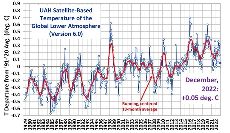
In this two-part series, I’m going to look at the latest official global GHCN thermometer (Tmax, Tmin) dataset (Version 4) to see if there is evidence of spurious warming from increasing urbanization effects over time. In the latest GHCN dataset version Tmax and Tmin are no longer provided separately, only their average (Tavg) is available.
Based upon what I’ve seen so far, I’m convinced that there is spurious warming remaining in the GHCN-based temperature data. The only question is, how much? That will be addressed in Part II.
The issue is important (obviously) because if observed warming trends have been overstated, then any deductions about the sensitivity of the climate system to anthropogenic greenhouse gas emissions are also overstated. (Here I am not going to go into the possibility that some portion of recent warming is due to natural effects, that’s a very different discussion for another day).
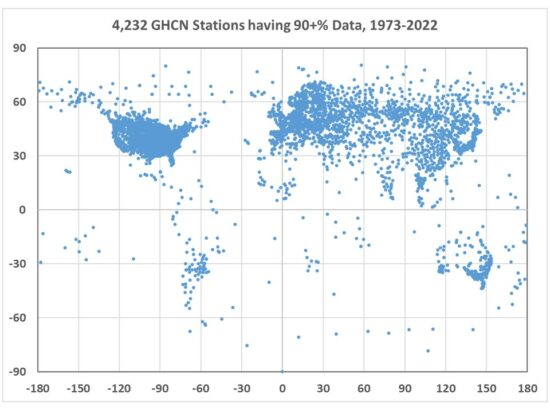
What I am going to show is based upon the global stations in the GHCN monthly dataset (downloaded January, 2023) which had sufficient data to produce at least 45 years of July data during the 50 year period, 1973-2022. The start years of 1973 is chosen for two reasons: (1) it’s when the separate dataset with hourly time resolution I’m analyzing had a large increase in the number of digitized records (remember, weather recording used to be a manual process onto paper forms, which someone has to digitize), and (2) the global Landsat-based urbanization data starts in 1975, which is close enough to 1973.
Because the Landsat measurements of urbanization are very high resolution, one must decide what spatial resolution should be used to relate to potential UHI effects. I have (somewhat arbitrarily) chosen averaging grid sizes of 3×3 km, 9×9 km, 21×21 km, and 45 x 45 km. In the global dataset I am getting the best results with the 21 x 21 km averaging of the urbanization data, and all results here will be shown for that resolution.
The resulting distribution of 4,232 stations (Fig. 1) shows that only a few countries have good coverage, especially the United States, Russia, Japan, and many European countries. Africa is poorly represented, as is most of South America.
I’ve analyzed the corresponding Landsat-based urban settlement diagnoses for all of these stations, which is shown in Fig. 2. That dataset covers a 40 year period, from 1975 to 2014. Here I’ve plotted the 40-year average level of urbanization versus the 40-year trend in urbanization.
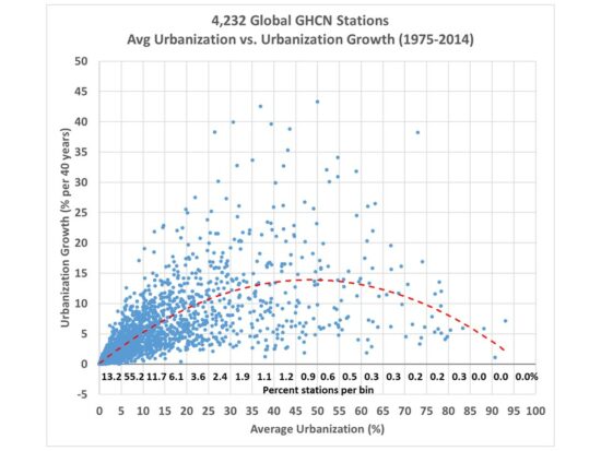
There are a few important and interesting things to note from Fig. 2.
- Few GHCN station locations are truly rural: 13.2% are less than 5% urbanized, while 68.4% are less than 10% urbanized.
- Virtually all station locations have experienced an increase in building, and none have decreased (which would require a net destruction of buildings, returning the land to its natural state).
- Greatest growth has been in areas not completely rural and not already heavily urbanized (see the curve fitted to the data). That is, very rural locations stay rural, and heavily urbanized locations have little room to grow anyway.
One might think that since the majority of stations are less than 10% urbanized that UHI effects should be negligible. But the seminal study by Oke (1973) showed that UHI warming is non-linear, with the most rapid warming occurring at the lowest population densities, with an eventual saturation of the warming at high population densities. I have previously showed evidence supporting this based upon updated global population density data that the greatest rate of spurious warming (comparing neighboring stations with differing populations) occurs at the lowest population densities. It remains to be seen whether this is also true of “built-up” measurements of human settlements (buildings rather than population density).
Average Urbanization or Urbanization Growth?
One interesting question is whether it is the trend in urbanization (growing amounts of infrastructure), or just the average urbanization that has the largest impact on temperature trends? Obviously, growth will have an impact. But what about towns and cities where there have been no increases in building, but still have had growth in energy use (which generates waste heat)? As people increasingly move from rural areas to cities, the population density can increase much faster than the number of buildings, as people live in smaller spaces and apartment and office buildings grow vertically without increasing their footprint on the landscape. There are also increases in wealth, automobile usage, economic productivity and consumption, air conditioning, etc., all of which can cause more waste heat production without an increase in population or urbanization.
In Part II I will examine how GHCN station temperature trends relate to station urbanization for a variety of countries, in both the raw (unadjusted) temperature data and in the homogenized (adjusted) data, and also look at how growth in urbanization compares to average urbanization.