…But the price per mile of EVs energy use is cheaper for the time being ($2 per gallon of gas equivalent)

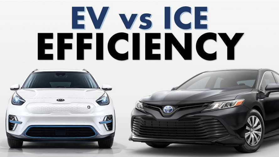
Photo credit: Insideevs.com.

Most of the electricity generated in the U.S. continues to come from fossil fuels (61% in 2021). This is not likely to change much in the future as electricity demand is increasing faster than renewables (20% of total in 2020 and 20.1% of total in 2021) can close the gap versus fossil fuels. Given that fact, it is interesting to ask the question:

Which uses fossil fuels more efficiently, an EV or ICE (internal combustion engine) vehicle?

Most of what you will read about EVs versus ICE vehicles discuss how EVs are more efficient at converting the energy they carry into motion (e.g. here, and here , and here, and here, etc.) but this is only part of the equation. The generation, transmission, and battery storage of electricity is very inefficient compared to the refining and transport of gasoline, and those inefficiencies each year add up to more than all of the gasoline consumed in the U.S.

EV Energy Usage per Mile

The average energy consumption of an EV vehicle is about 0.35 kWh per mile. At the U.S. average electricity price of $0.145 per kWh in June 2022, and assuming the 2021 average new car fuel economy of 39 mpg, this makes the ICE-equivalent fuel price of an EV $1.98 per gallon of gasoline. With the U.S. average price of gas now over $5.00 a gallon, this by itself (ignoring the many other considerations, discussed below) makes the EV attractive for month-to-month savings on fuel purchases.

But since most of this electricity still comes from fossil fuels, we must factor in the efficiency with which electricity is generated and transmitted and stored in the EV’s battery. This is how we can answer the question, Which uses fossil fuels more efficiently, an EV or ICE (internal combustion engine) vehicle?

The generation of electricity is pretty inefficient with efficiencies ranging 33% from coal and 42% from natural gas. As we continue to transition away from coal to natural gas, I will use the 42% number. Next, at least 6.5% is lost in transmission and distribution. Finally, 12% of the electricity is lost in charging of the EV battery. Taken together, these losses add up to the 0.35 kWh per mile energy efficiency of an EV increasing to 1.0 kWh per mile in terms of fossil energy being used.

ICE Energy Usage per Mile

How does the internal combustion engine stack up against the EV in terms of efficiency of fossil fueled energy use?

A gallon of gas contains 33.7 kWh of energy. But like the generation of electricity, it takes energy to extract that gallon of gas from petroleum. However, the refining process is very energy efficient (about 90%), so it takes (33.7/0.9=) 37.44 kWh of energy to obtain that 33.7 kWh of energy is a gallon of gas. At the 39 mpg gas mileage of 2021 cars, this gives an energy economy number of 0.96 kWh per mile driven, which is just below the 1.0 kWh fossil fuel energy usage of an EV. With advertised fuel economy of 48 to 60 mpg, hybrid vehicles (which are gasoline powered) would thus have an advantage over EVs.

Other Considerations

Of course, the main reason EVs are being pushed on the American people (through subsidies and stringent CAFE standards) is the reduction in CO2 emissions that will occur, assuming more of our electricity comes from non-fossil fuel sources in the future. I personally have no interest in owning one because I want the flexibility of travelling long distances in a single day.

There is also the issue of the large amount of additional natural resources, and associated pollution, required to make millions of EV batteries.

Furthermore, the electrical grid will need to be expanded to provide the increase in electricity needed. This greater electricity demand, along with the high cost of wind and solar energy, might well make the fuel cost advantage of the EV disappear in the coming years.

Finally, a portion of the true price of a new EV is hidden through subsides (which the taxpayer pays for) and high CAFE fuel economy regulations, which require auto manufacturers not meeting the standard to pay companies like Tesla, a cost which is passed on to the consumer through higher prices on ICE cars and (especially) trucks.

As early as today at noon EDT an Astra rocket will launch the first two of six small CubeSats into tropical orbits at 550 km altitude from Cape Canaveral (video coverage here). Those satellites, named the TROPICS mission, will carry microwave radiometers operating at relatively high frequencies, from 90 to 205 GHz. They will measure precipitation-size ice particles in the upper reaches of tropical storms (at 90 and 205 GHz), and provide temperature (118 GHz channels) and humidity profiles (183 GHz channels) in the environment surrounding, and inside the warm cores of those storms.

History
The use of microwave radiometers in space to observe the Earth was first proposed by German meteorologist Konrad Buettner in 1963. By the late 1960s aircraft missions were being flown by NASA and the U.S. Weather Bureau to demonstrate the technology.

In the early 1970s NASA/Goddard was the leader in the construction and flight of the first spaceborne microwave radiometers to demonstrate the measurement of precipitation and sea ice with the single-frequency ESMR instruments operating at 19.35 and 37 GHz.

Later, JPL developed the SMMR instrument that provided measurements from 6.6 to 37 GHz starting in late 1978 on the Nimbus-7 satellite. That instrument allowed me as a post-doc at UW-Madison to demonstrate the ability to measure precipitation over land by isolating the ice scattering signature at 37 GHz, which gave me my first peer-reviewed paper (a cover article in Nature) and led to several more papers describing severe thunderstorm detection and rainfall measurement. It is this ice scattering signature that will be exploited as part of the TROPICS mission.

The field of researchers in satellite passive microwave remote sensing up to the Nimbus-7 SMMR period was pretty small. It was the 1987 launch of the first SSM/I instrument on a DoD DMSP satellite that got many more researchers involved in using satellite microwave measurements. The unusual inclusion of higher-frequency 85.5 GHz channels on SSM/I exploited the ice signature that Dick Savage (UW-Madison) also documented along with Jim Weinman.

Meanwhile, the JPL-built MSU instruments were providing atmospheric temperature profile data since late 1978 in the 60 GHz oxygen absorption complex, mostly for data input to weather forecast models. Later, NOAA and NASA/GSFC developed the higher-resolution AMSU instruments, first launched in 1998, which still provide global atmospheric temperature information.

It was around 1990 that John Christy and I demonstrated that the MSU/AMSU series of temperature-profiling instruments could provide a relatively stable long-term record of global atmospheric temperatures for monitoring of climate change. While I had helped with the early planning of NASA’s TRMM satellite to monitor tropical rainfall, I chose to change my career focus from precipitation monitoring to temperature monitoring, and declined to become part of the official TRMM Team. I would still become the U.S. Science Team leader for the AMSR-E instrument (built by Japan), which like SSM/I measured a wide variety of parameters, but my time would be increasingly devoted to the global temperature monitoring effort.

The radical TROPICS approach to tropical cyclone monitoring
One of the main advantages of passive microwave measurements is the ability to see through many clouds (especially cirrus). Unfortunately, satellite passive microwave radiometry has always struggled with poor spatial resolution. The beamwidth of a diffraction-limited microwave antenna increases with the wavelength of radiation being measured, so large antennas are required to obtain high resolution on the Earth’s surface. Or, shorter wavelength (higher frequency) channels need to be utilized. The trouble with high frequencies, though, is that clouds become more opaque as the frequency increases. If you increase the frequency too high you move into the infrared, and we already have geostationary satellites providing those data on a continuous basis.

The TROPICS approach employs both a lower altitude (550 km compared to 700 to 850 km from other satellites) and higher frequencies (90 to 205 GHz) to improve spatial resolution. Microwave circuit electronics have improved in sensitivity and noise and have been reduced in size to the point that the very small and lightweight CubeSat architecture can be used. The TROPICS satellites use 3 CubeSat modules, making the satellite bus only (approximately) 4 x 4 x 12 inches in size. The mission’s Principal Investigator, William Blackwell at MIT’s Lincoln Lab has been spearheading this new, smaller microwave radiometer concept. The temperature sounding utilizes the 118 GHz oxygen absorption complex, rather than 60 GHz (as with the AMSUs) which improves spatial resolution by a factor of two.

Such small satellites can be launched in batches with smaller rockets, which reduces cost. It also aligns with NASA’s overriding interest in satellite technology advancement. With six of these satellites in a low-inclination (30 deg) orbit, quasi-hourly coverage (on average) of tropical cyclones is anticipated.

What will forecasters do with the data?
Many years ago I visited both the National Hurricane Center (Florida) and the Joint Typhoon Warning Center (Hawaii) to promote the use of passive microwave measurements of tropical storms. Since then, several researchers (e.g. Chris Velden and Mark DeMaria) have worked tirelessly with these centers to establish procedures for passive microwave monitoring of tropical cyclones.

I suspect the measurements will mostly be used to better isolate where a tropical depression or storm might be forming since the microwave measurements penetrate most cirrus cloud cover and can better reveal the low-level swirl of clouds marking the circulation center. Regarding the monitoring of a tropical cyclone’s warm core (what causes the intense low pressure at the surface) it isn’t until the storm comes close to hurricane intensity (65 knot maximum sustain surface winds) that the warm core can be reliably measured by TROPICS satellites. Also, the 27 km (best case) spatial resolution for the 118 GHz temperature sounding channels is still a little too coarse to avoid precipitation contamination (a cold signature) of the warm core signature that typifies tropical cyclones. Nevertheless, I’m sure researchers will find clever ways to isolate the warm core signature, just as we did in Spencer et al. (2001) using AMSU satellite data at 50 km resolution.

There will no doubt be some new capabilities that emerge as data are gathered from these satellites. For example, a large hurricane with frequent coverage by TROPICS satellites might reveal rapid deepening of the storm through a stronger warm core signature. In the absence of Hurricane Hunter flights into the storms, storm intensity is still largely based upon weather satellite visible and infrared cloud features, which is a rather indirect (but surprisingly accurate) technique that has a long history. TROPICS offers the chance to have a more physics-based measurement of hurricane intensity than through cloud appearance alone. Also, since data will continuously be collected over the entire tropical latitude belt, a wide variety of other applications will arise.

Let’s hope the Astra launch (maybe today) will be successful. So far, there have only been two successful Astra launches out of eight attempts (one rather dramatic failure is shown below). Fingers crossed.

The Version 6.0 global average lower tropospheric temperature (LT) anomaly for May, 2022 was +0.17 deg. C, down from the April, 2022 value of +0.26 deg. C.

The linear warming trend since January, 1979 still stands at +0.13 C/decade (+0.12 C/decade over the global-averaged oceans, and +0.18 C/decade over global-averaged land).

Various regional LT departures from the 30-year (1991-2020) average for the last 17 months are:

YEAR MO GLOBE NHEM. SHEM. TROPIC USA48 ARCTIC AUST 
2021 01  0.12  0.34 -0.09 -0.08  0.36  0.50 -0.52
2021 02  0.20  0.31  0.08 -0.14 -0.66  0.07 -0.27
2021 03 -0.01  0.12 -0.14 -0.29  0.59 -0.78 -0.79
2021 04 -0.05  0.05 -0.15 -0.28 -0.02  0.02  0.29
2021 05  0.08  0.14  0.03  0.06 -0.41 -0.04  0.02
2021 06 -0.01  0.30 -0.32 -0.14  1.44  0.63 -0.76
2021 07  0.20  0.33  0.07  0.13  0.58  0.43  0.80
2021 08  0.17  0.26  0.08  0.07  0.32  0.83 -0.02
2021 09  0.25  0.18  0.33  0.09  0.67  0.02  0.37
2021 10  0.37  0.46  0.27  0.33  0.84  0.63  0.06
2021 11  0.08  0.11  0.06  0.14  0.50 -0.43 -0.29
2021 12  0.21  0.27  0.15  0.03  1.63  0.01 -0.06
2022 01  0.03  0.06  0.00 -0.24 -0.13  0.68  0.09
2022 02 -0.00  0.01 -0.02 -0.24 -0.05 -0.31 -0.50
2022 03  0.15  0.27  0.02 -0.08  0.22  0.74  0.02
2022 04  0.26  0.35  0.18 -0.04 -0.26  0.45  0.60
2022 05  0.17  0.24  0.10  0.01  0.59  0.22  0.19