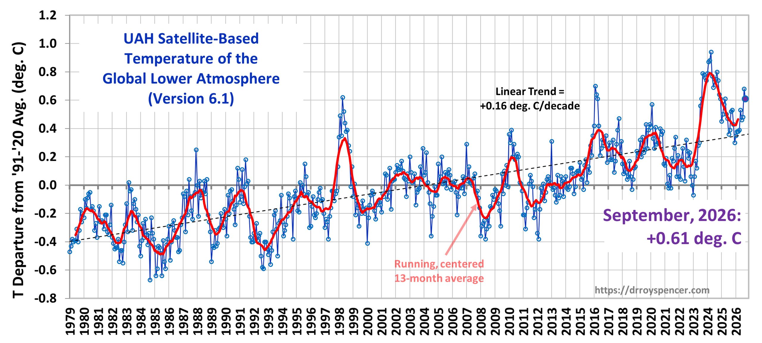
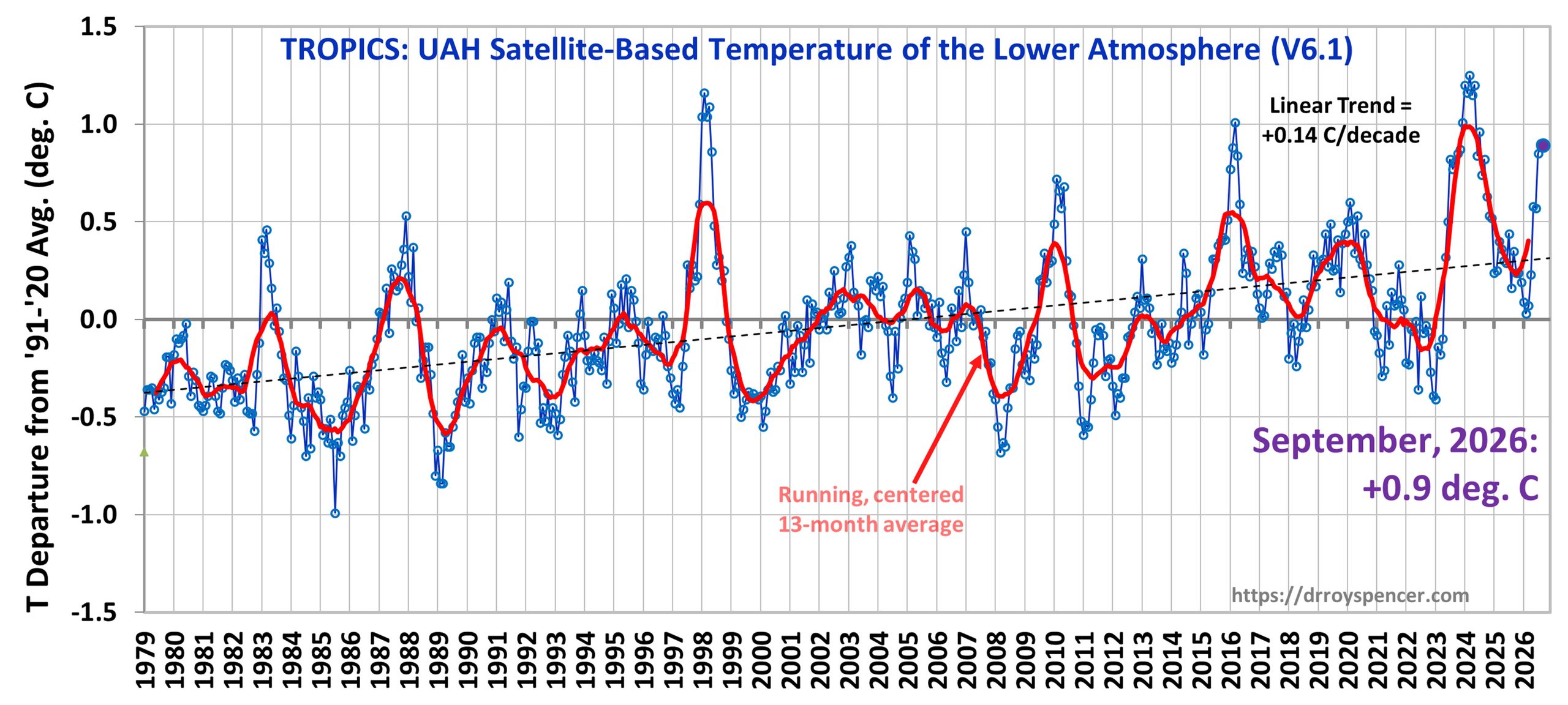
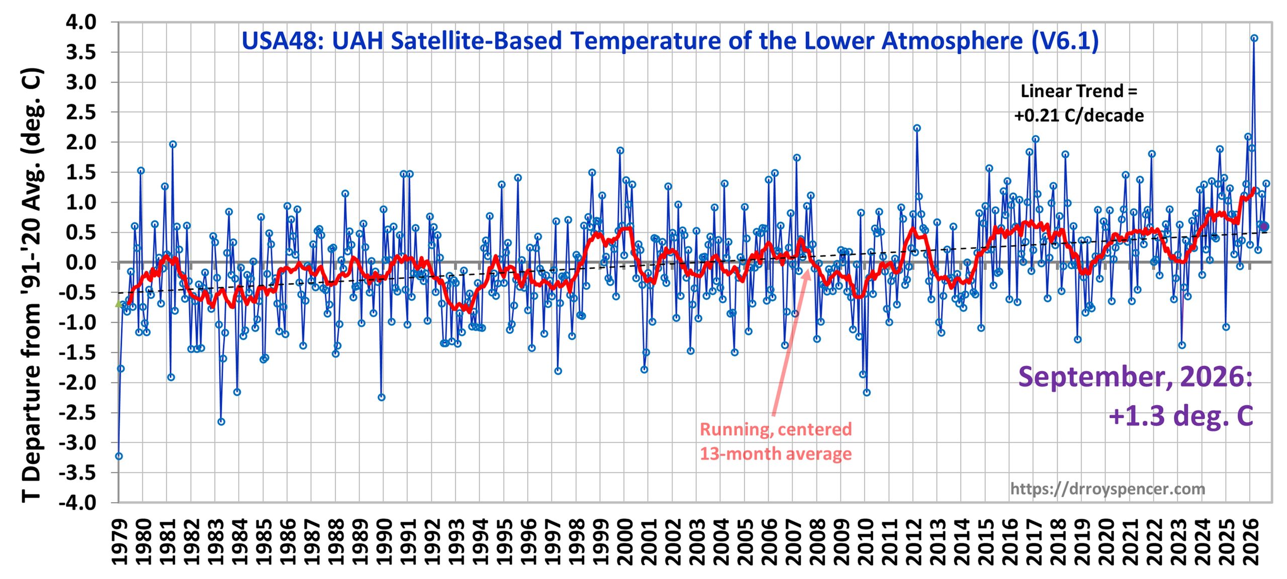
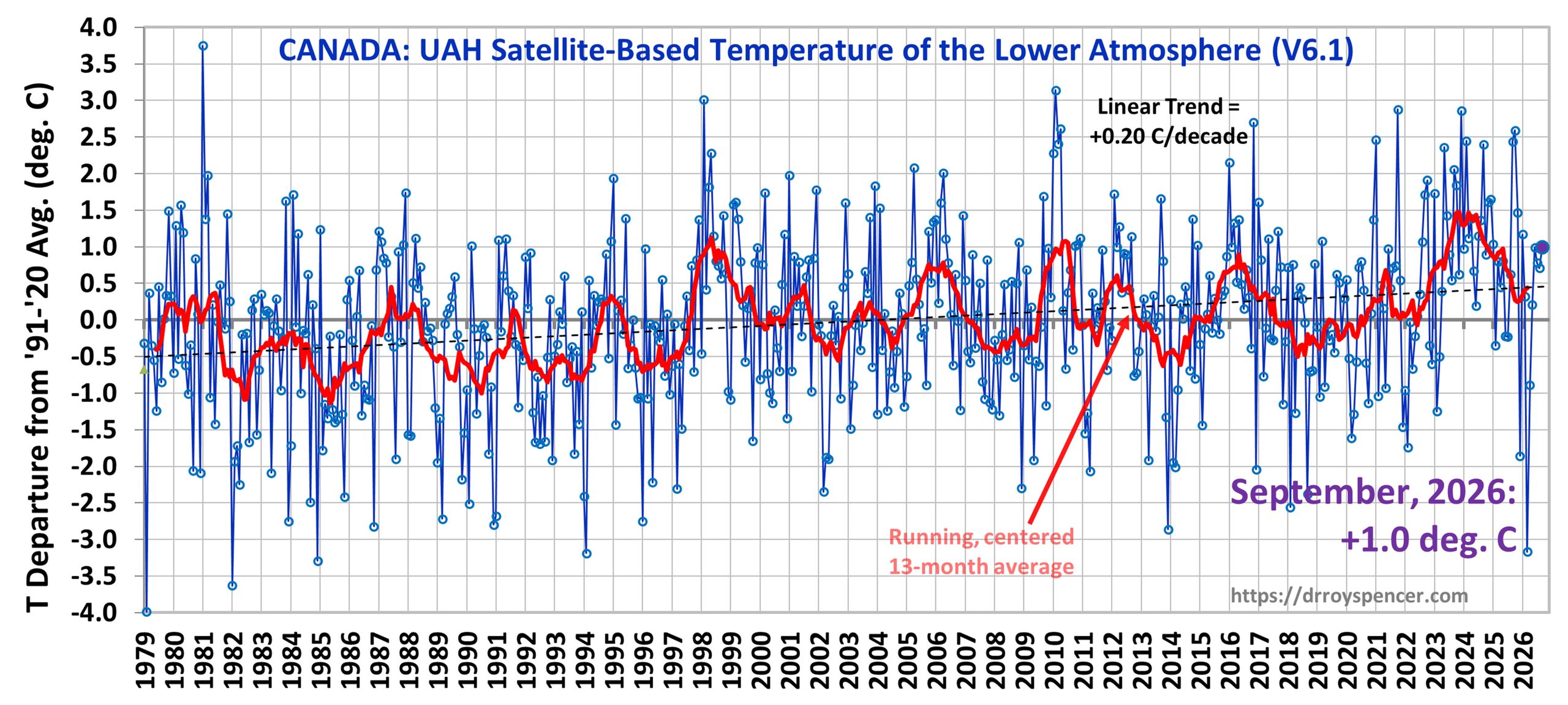
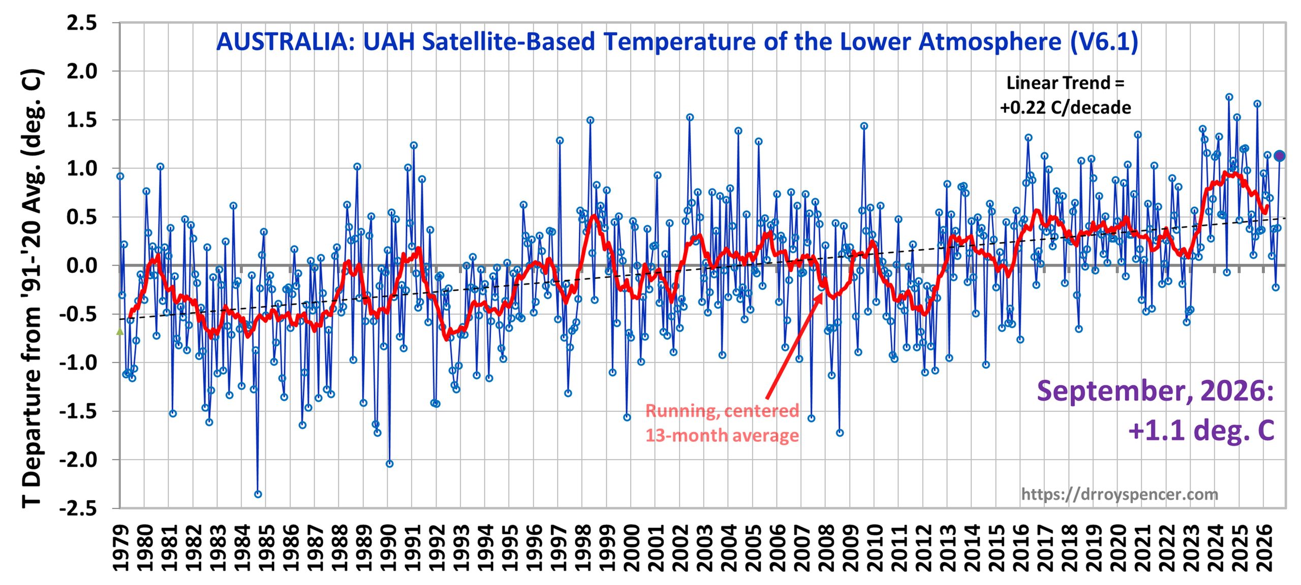
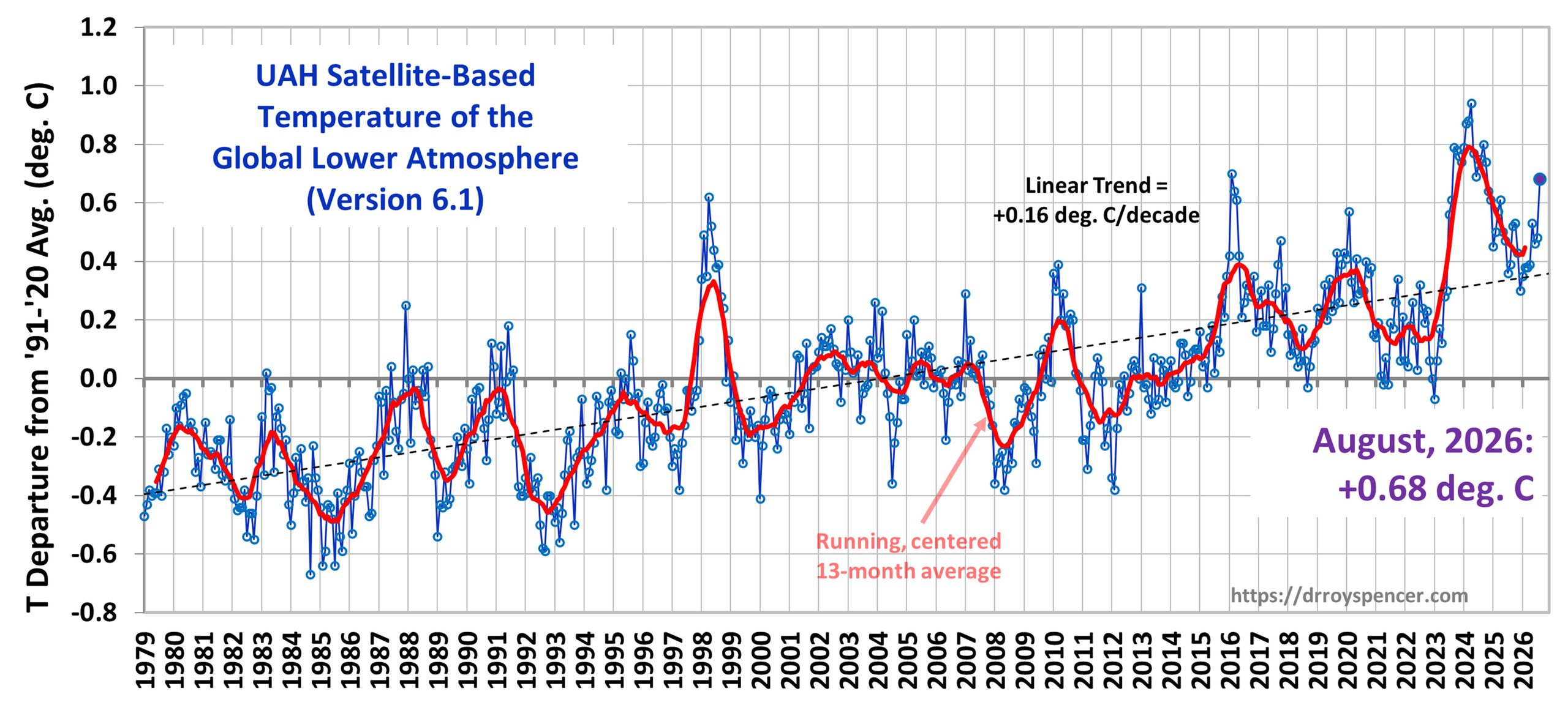
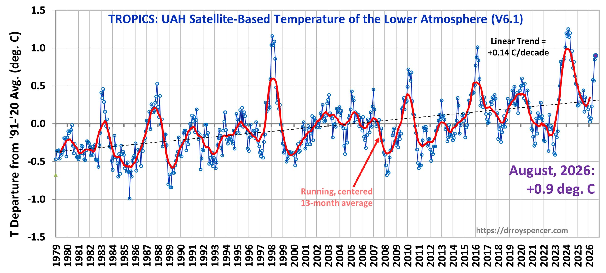
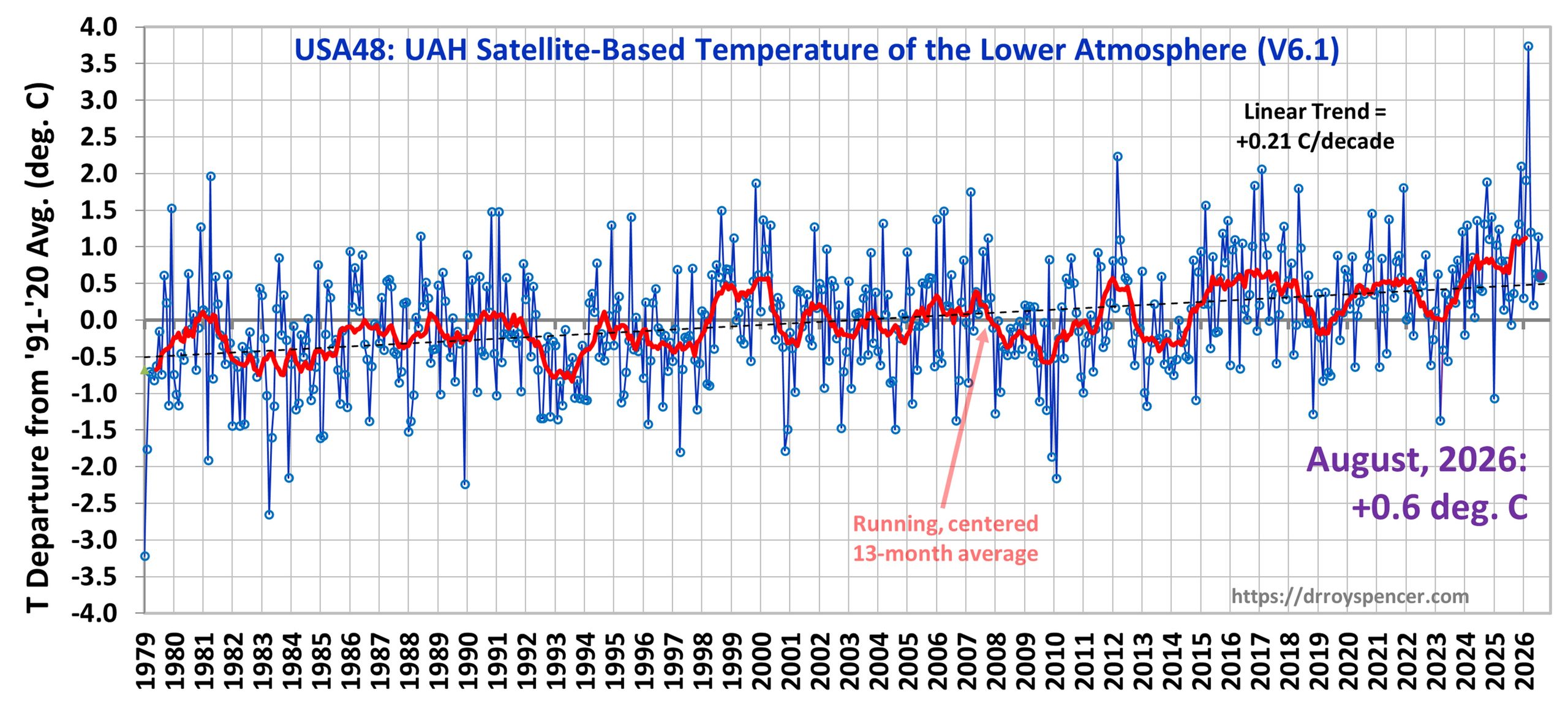
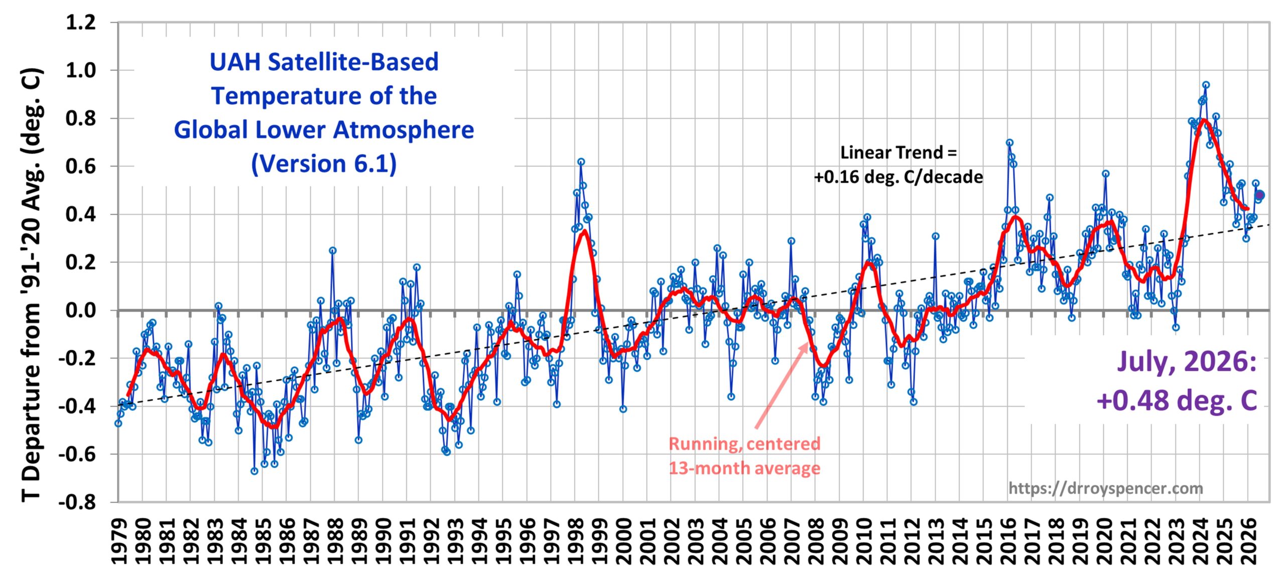
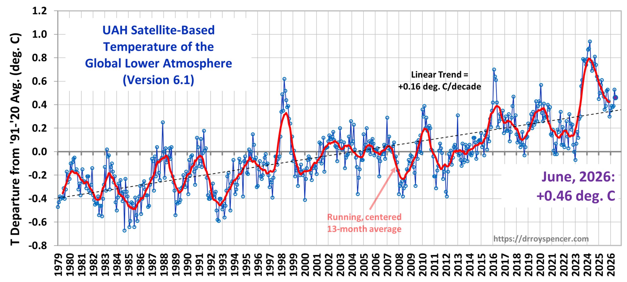
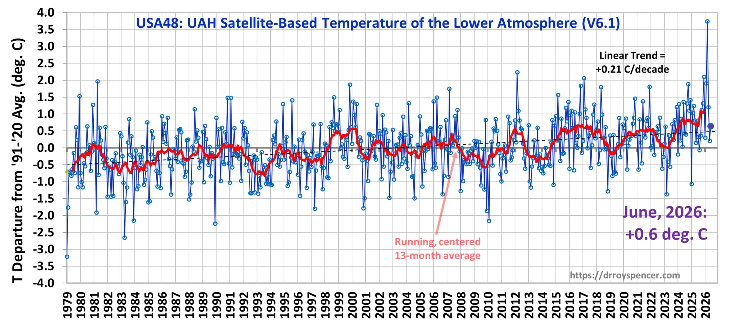
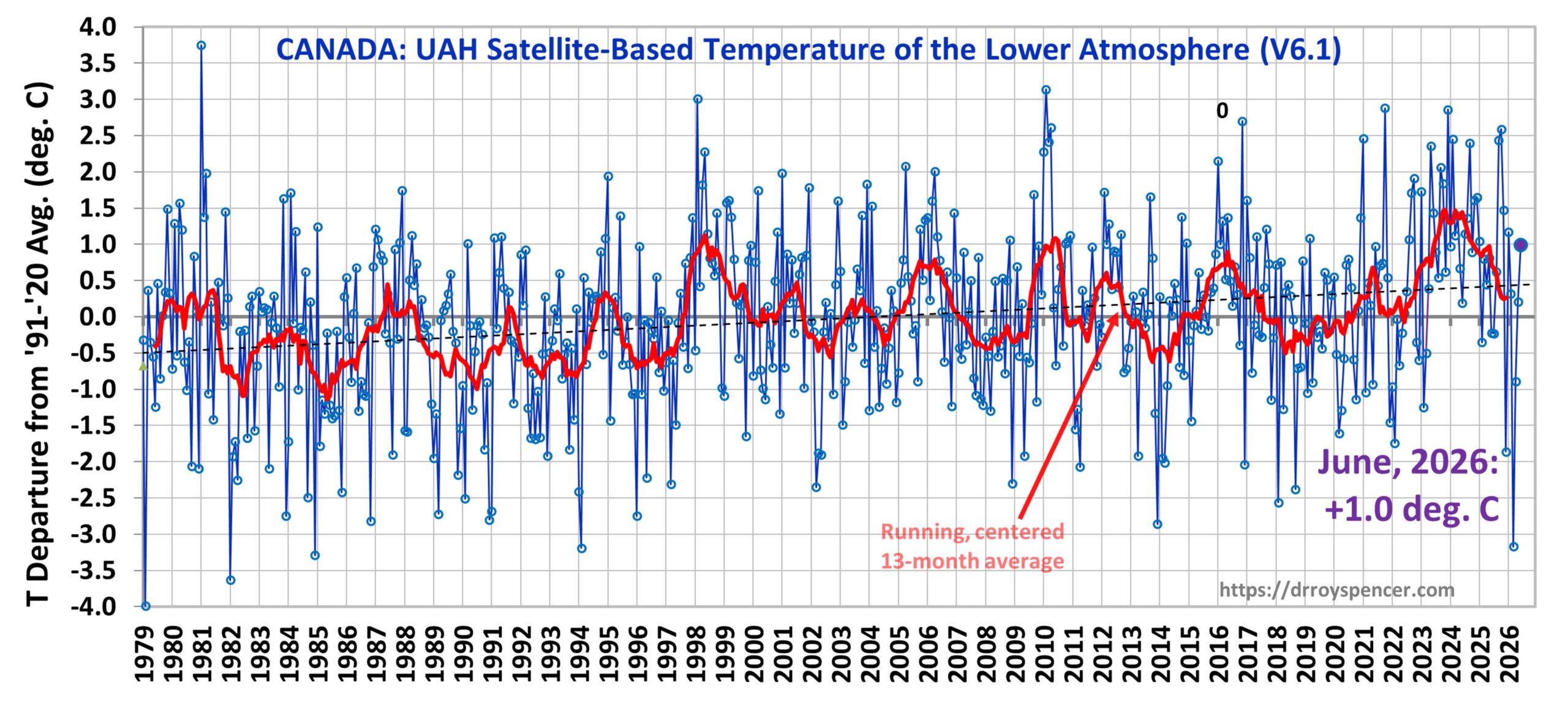
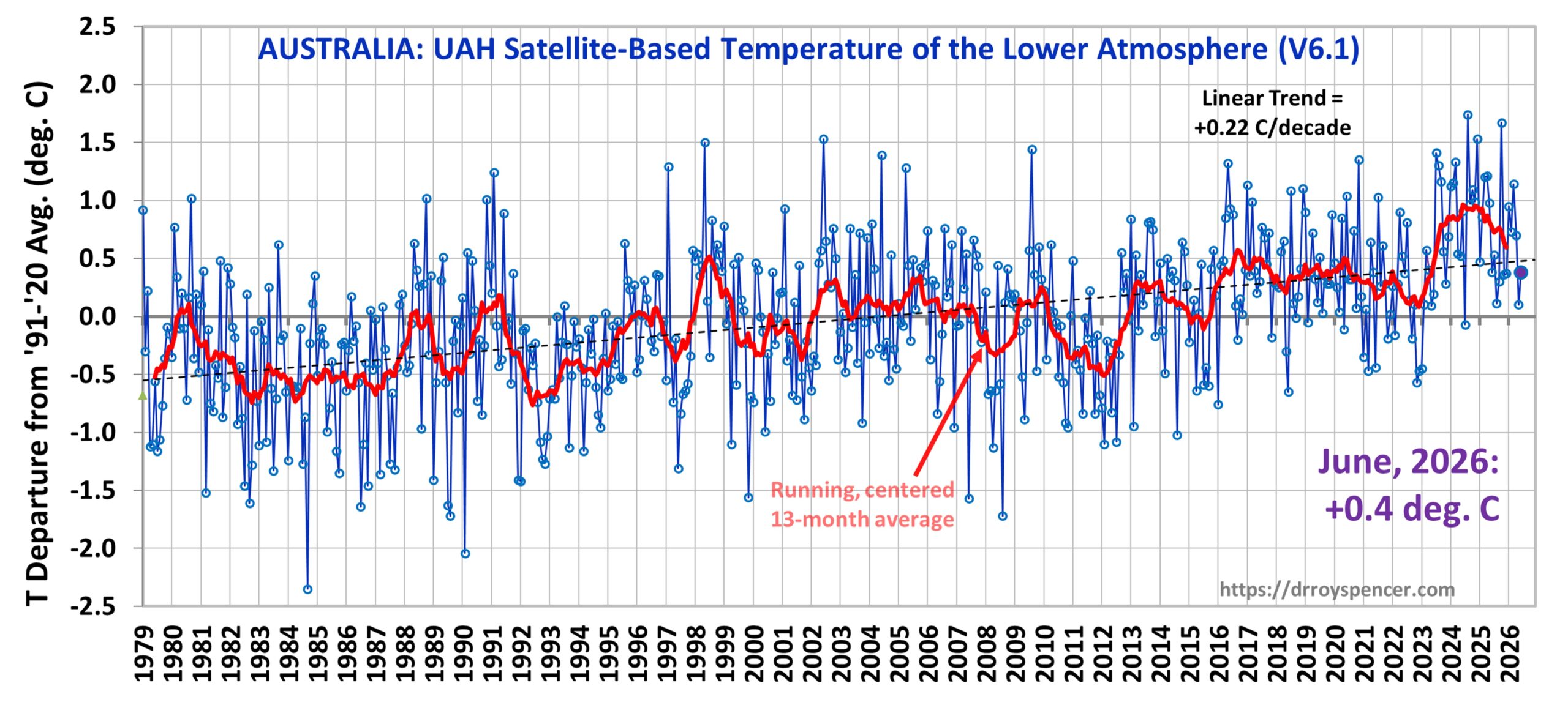
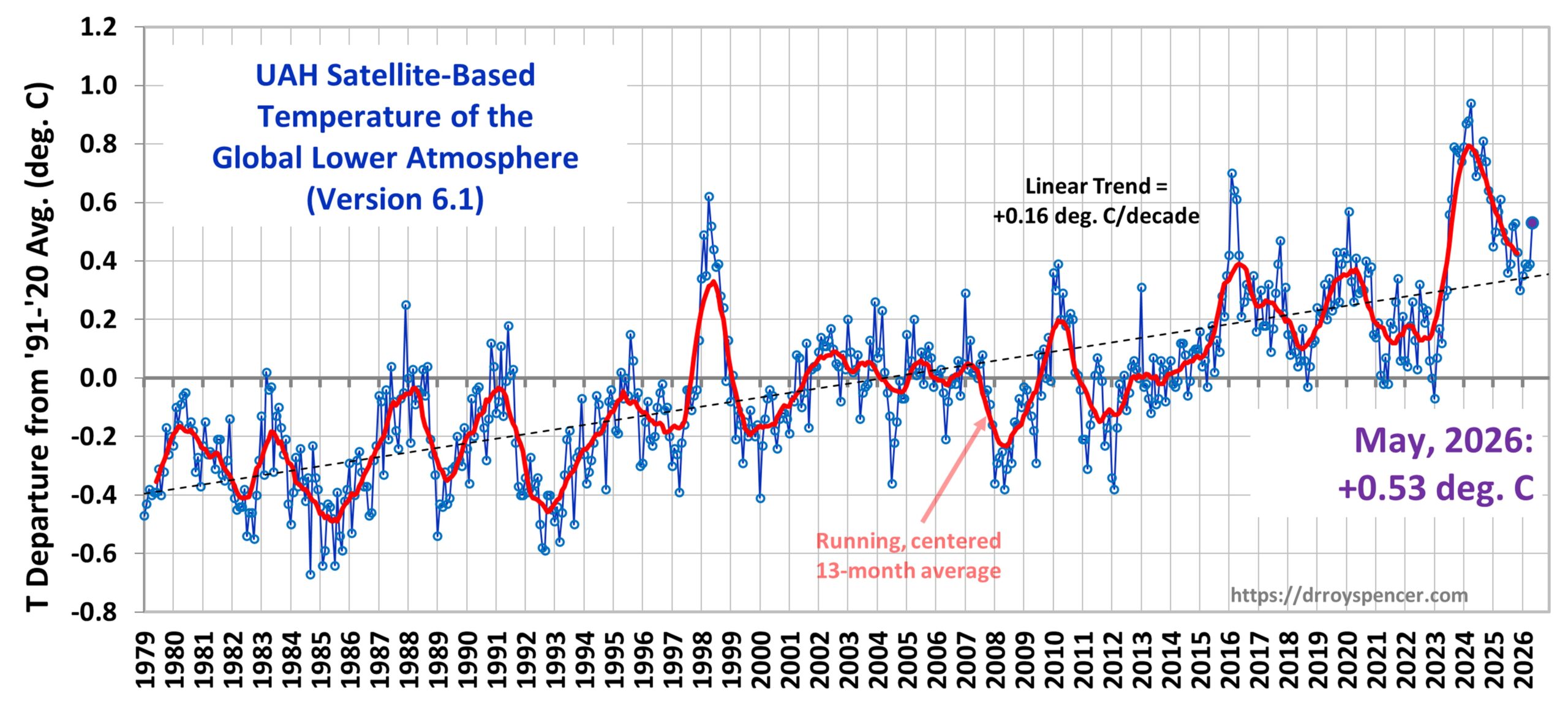
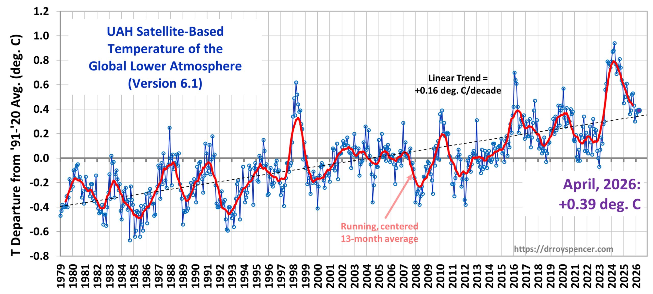
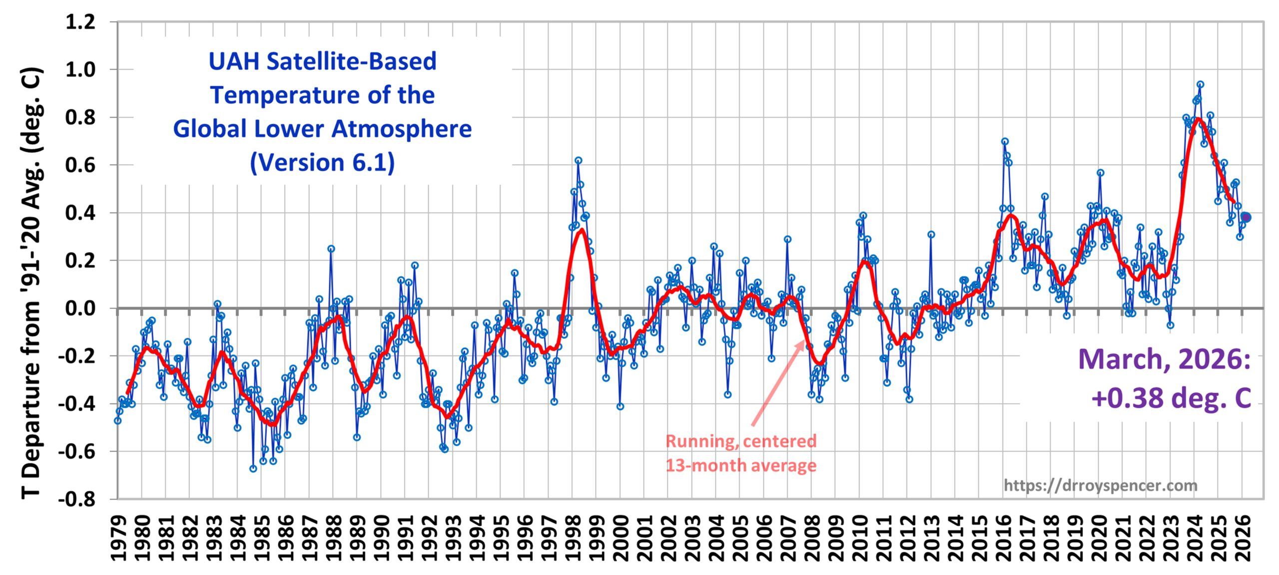
The Version 6.1 global average lower tropospheric temperature (LT) anomaly for September, 2026 was +0.61 deg. C departure from the 1991-2020 mean, down from the August, 2026 value of +0.68 deg. C.
The Version 6.1 global area-averaged linear temperature trend (January 1979 through September 2026) remains at +0.16 deg/ C/decade (+0.22 C/decade over land, +0.13 C/decade over oceans).
The following table lists various regional Version 6.1 LT departures from the 30-year (1991-2020) average for the last 33 months (record highs are in red).
Year
Mon
Globe
NHem
SHem
Tropic
US48
Arctic
Aust.
Can.
2024
Jan
+0.80
+1.02
+0.57
+1.20
-0.19
+0.40
+1.12
+0.97
2024
Feb
+0.88
+0.94
+0.81
+1.16
+1.31
+0.85
+1.16
+2.45
2024
Mar
+0.88
+0.96
+0.80
+1.25
+0.22
+1.05
+1.34
+1.12
2024
Apr
+0.94
+1.12
+0.76
+1.15
+0.86
+0.88
+0.54
+1.39
2024
May
+0.77
+0.77
+0.78
+1.20
+0.04
+0.20
+0.52
+0.67
2024
June
+0.69
+0.78
+0.60
+0.85
+1.36
+0.63
+0.91
+0.19
2024
July
+0.73
+0.86
+0.61
+0.96
+0.44
+0.56
-0.07
+1.15
2024
Aug
+0.75
+0.81
+0.69
+0.74
+0.40
+0.88
+1.75
+1.36
2024
Sep
+0.81
+1.04
+0.58
+0.82
+1.31
+1.48
+0.98
2024
Oct
+0.75
+0.89
+0.60
+0.63
+1.89
+0.81
+1.09
+0.89
2024
Nov
+0.64
+0.87
+0.40
+0.53
+1.11
+0.79
+1.00
+1.61
2024
Dec
+0.61
+0.75
+0.47
+0.52
+1.41
+1.12
+1.54
+1.65
2025
Jan
+0.45
+0.70
+0.21
+0.24
-1.07
+0.74
+0.48
+1.04
2025
Feb
+0.50
+0.55
+0.45
+0.26
+1.03
+2.10
+0.87
-0.35
2025
Mar
+0.57
+0.73
+0.41
+0.40
+1.24
+1.23
+1.20
+0.80
2025
Apr
+0.61
+0.76
+0.46
+0.36
+0.81
+0.85
+1.21
+0.45
2025
May
+0.50
+0.45
+0.55
+0.30
+0.15
+0.75
+0.98
+0.81
2025
June
+0.48
+0.48
+0.47
+0.30
+0.80
+0.05
+0.39
-0.22
2025
July
+0.36
+0.49
+0.23
+0.45
+0.32
+0.40
+0.53
-0.23
2025
Aug
+0.39
+0.39
+0.39
+0.16
-0.06
+0.82
+0.11
+0.62
2025
Sep
+0.53
+0.56
+0.49
+0.35
+0.38
+0.77
+0.30
+2.44
2025
Oct
+0.53
+0.52
+0.55
+0.24
+1.12
+1.42
+1.67
+2.59
2025
Nov
+0.43
+0.59
+0.27
+0.24
+1.32
+0.78
+0.36
+1.47
2025
Dec
+0.30
+0.45
+0.15
+0.19
+2.10
+0.32
+0.37
-1.86
2026
Jan
+0.35
+0.51
+0.19
+0.09
+0.30
+1.40
+0.95
+1.17
2026
Feb
+0.39
+0.54
+0.23
+0.03
+1.91
-0.48
+0.73
+0.32
2026
Mar
+0.38
+0.33
+0.42
+0.07
+3.74
-0.48
+1.14
-3.17
2026
Apr
+0.39
+0.43
+0.34
+0.23
+1.20
+0.30
+0.70
-0.89
2026
May
+0.53
+0.46
+0.60
+0.58
+0.21
+0.34
+0.10
+0.21
2026
June
+0.46
+0.54
+0.38
+0.57
+0.64
+1.01
+0.38
+0.99
2026
July
+0.48
+0.68
+0.27
+0.85
+1.14
+0.53
-0.22
+0.78
2026
Aug
+0.68
+0.76
+0.59
+0.90
+0.60
+0.80
+0.39
+0.71
2026
Sep
+0.61
+0.78
+0.44
+0.89
+1.32
+0.80
+1.13
+0.99
Year
Mon
Globe
NHem
SHem
Tropic
US48
Arctic
Aust.
Can.
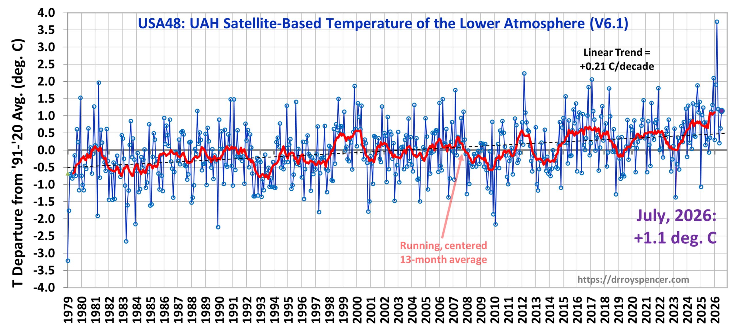
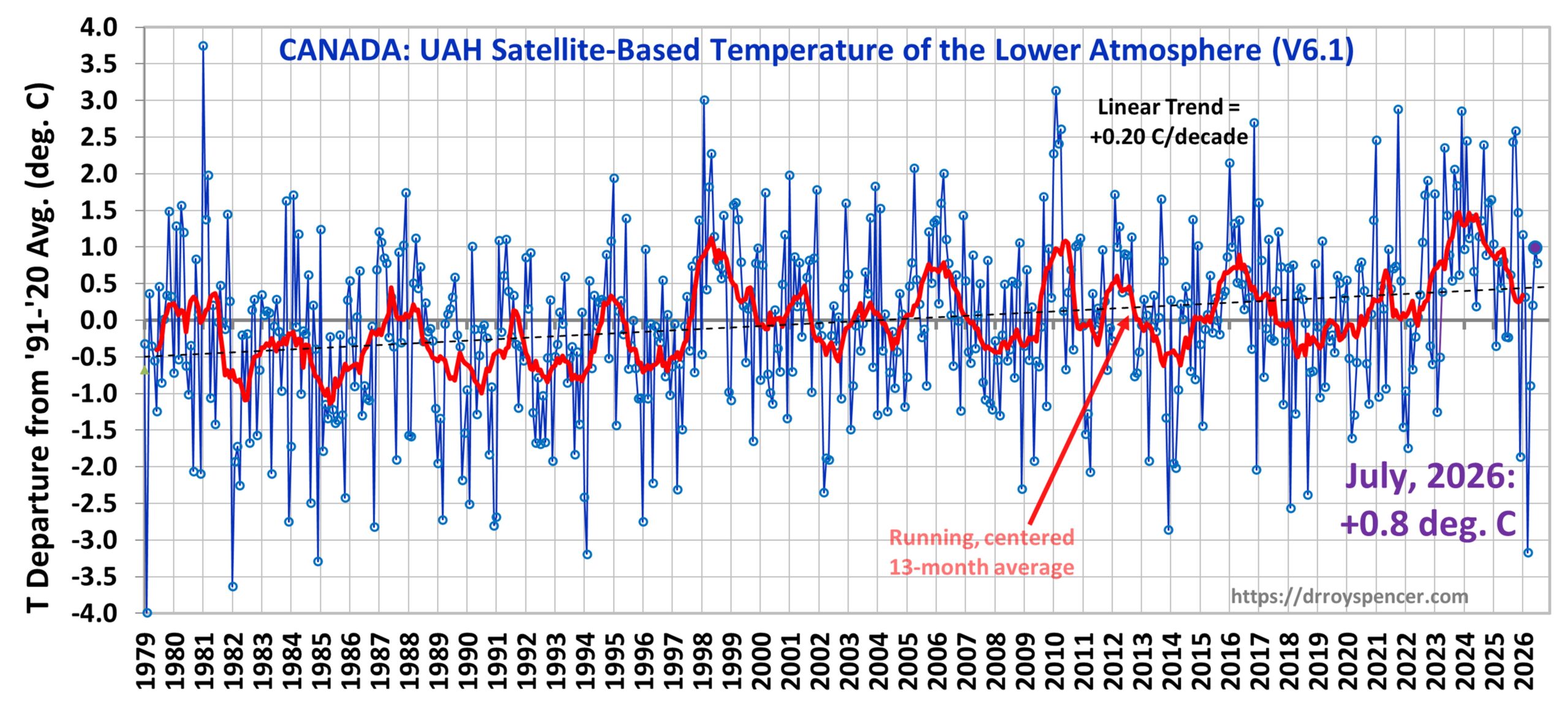
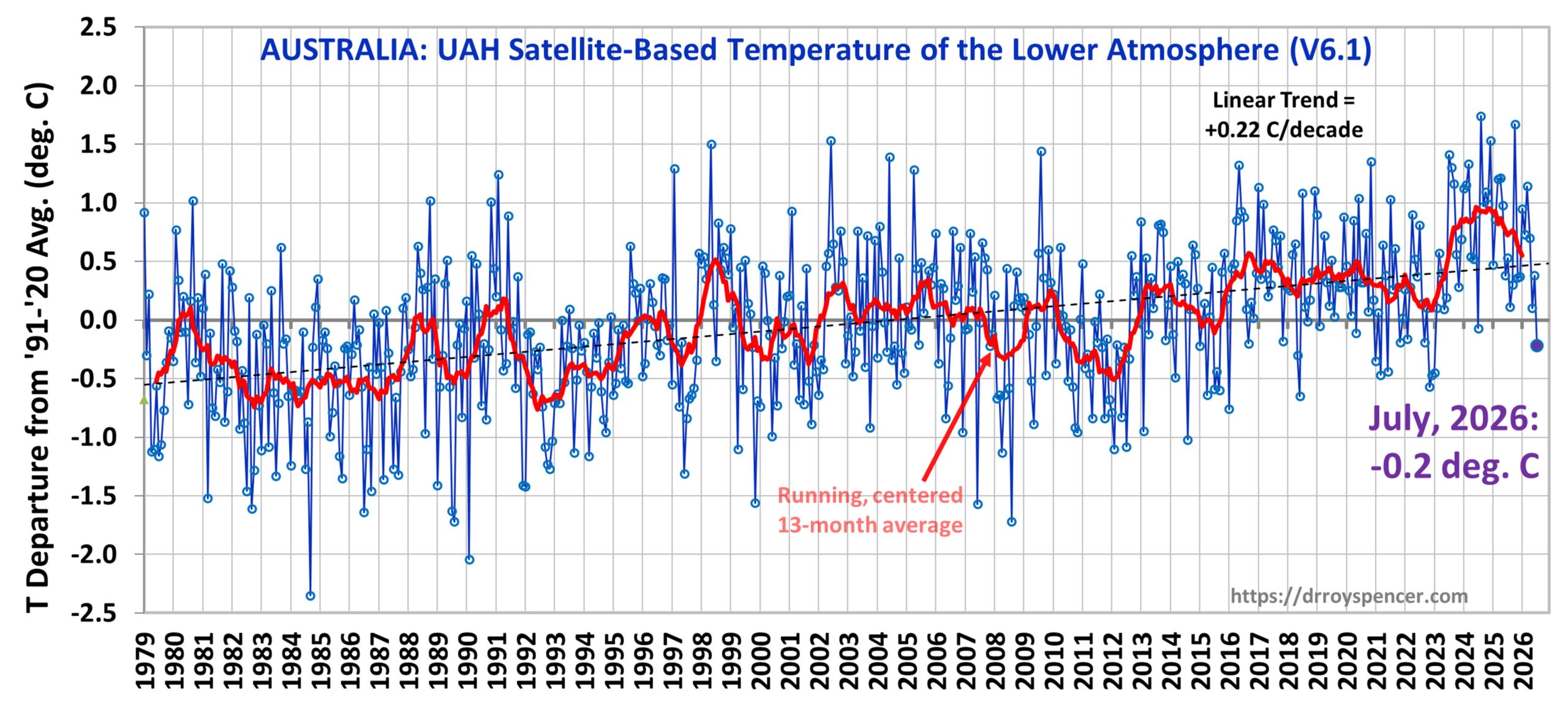
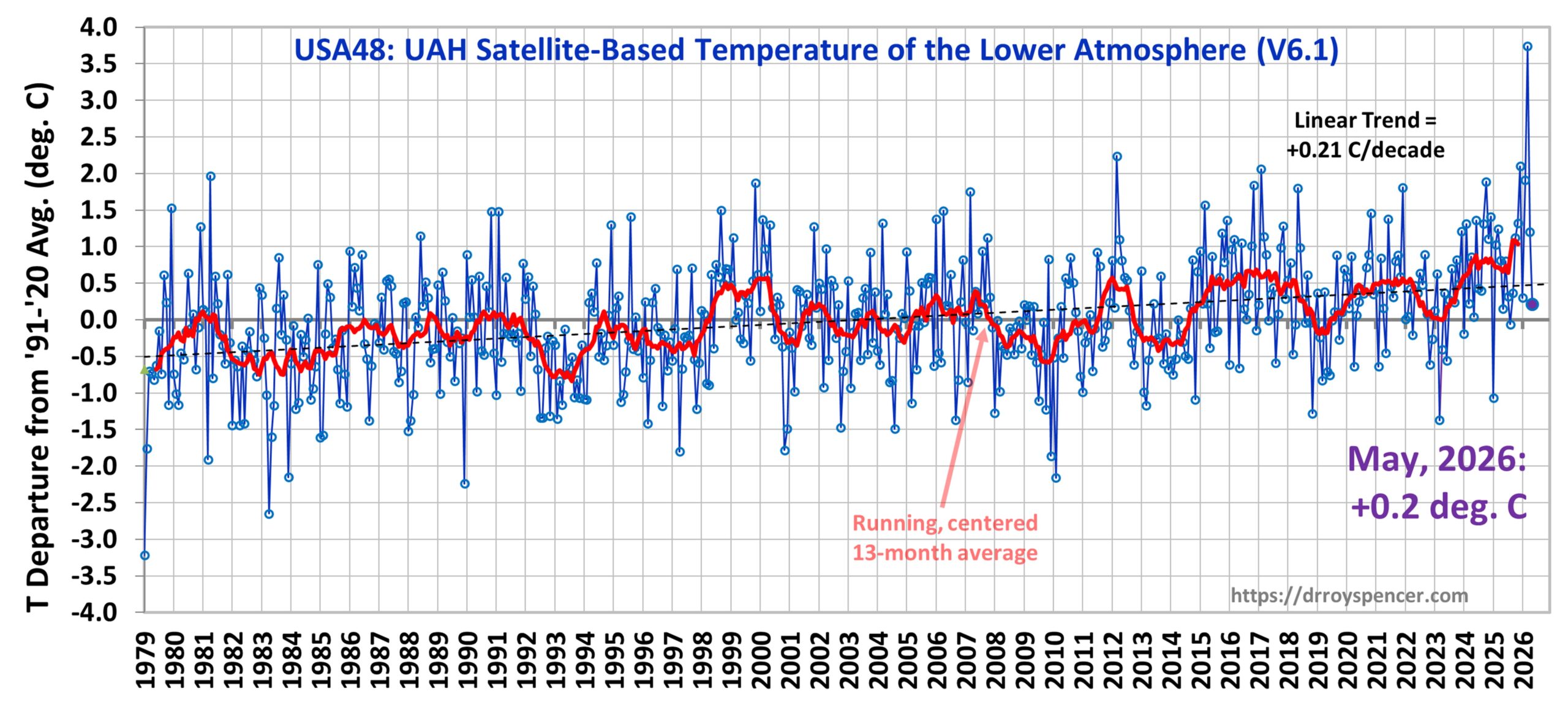
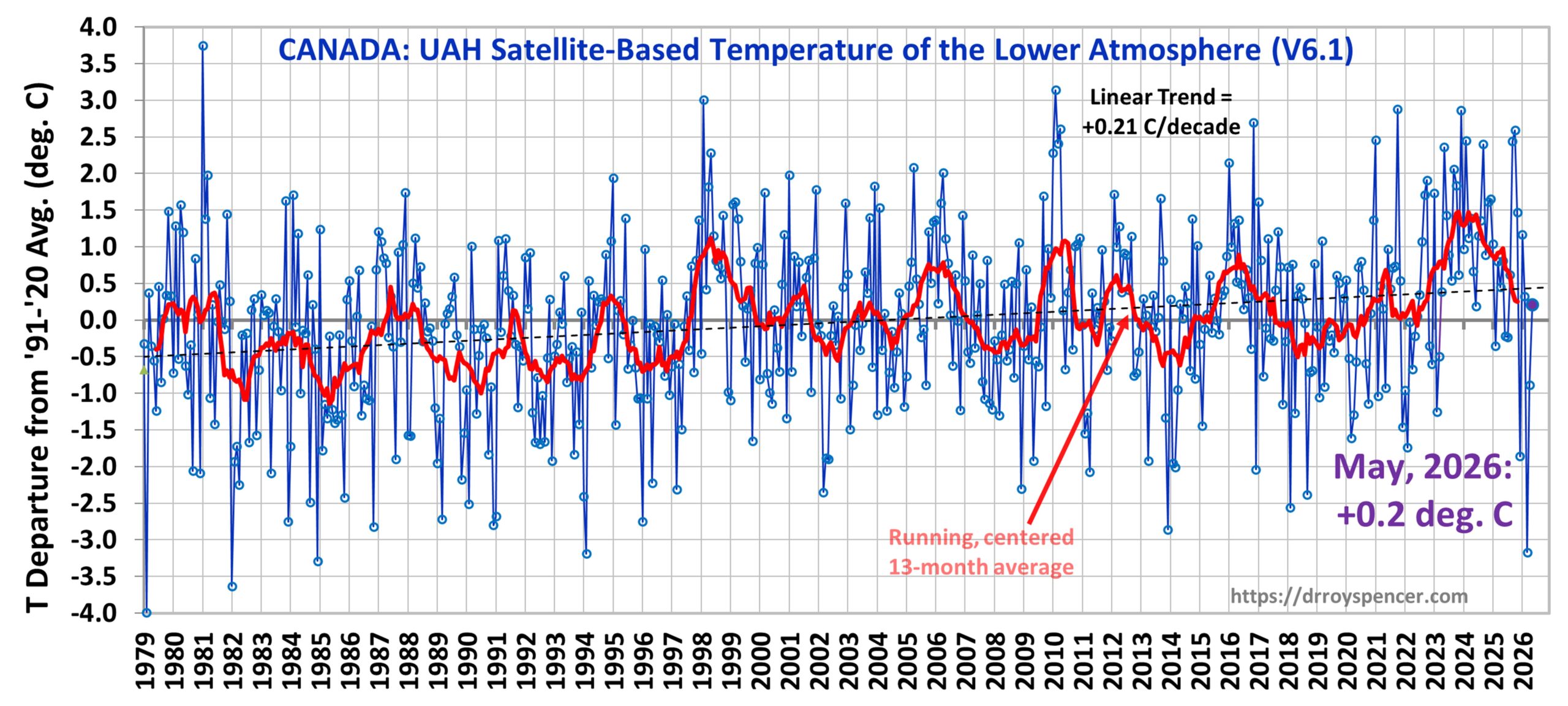
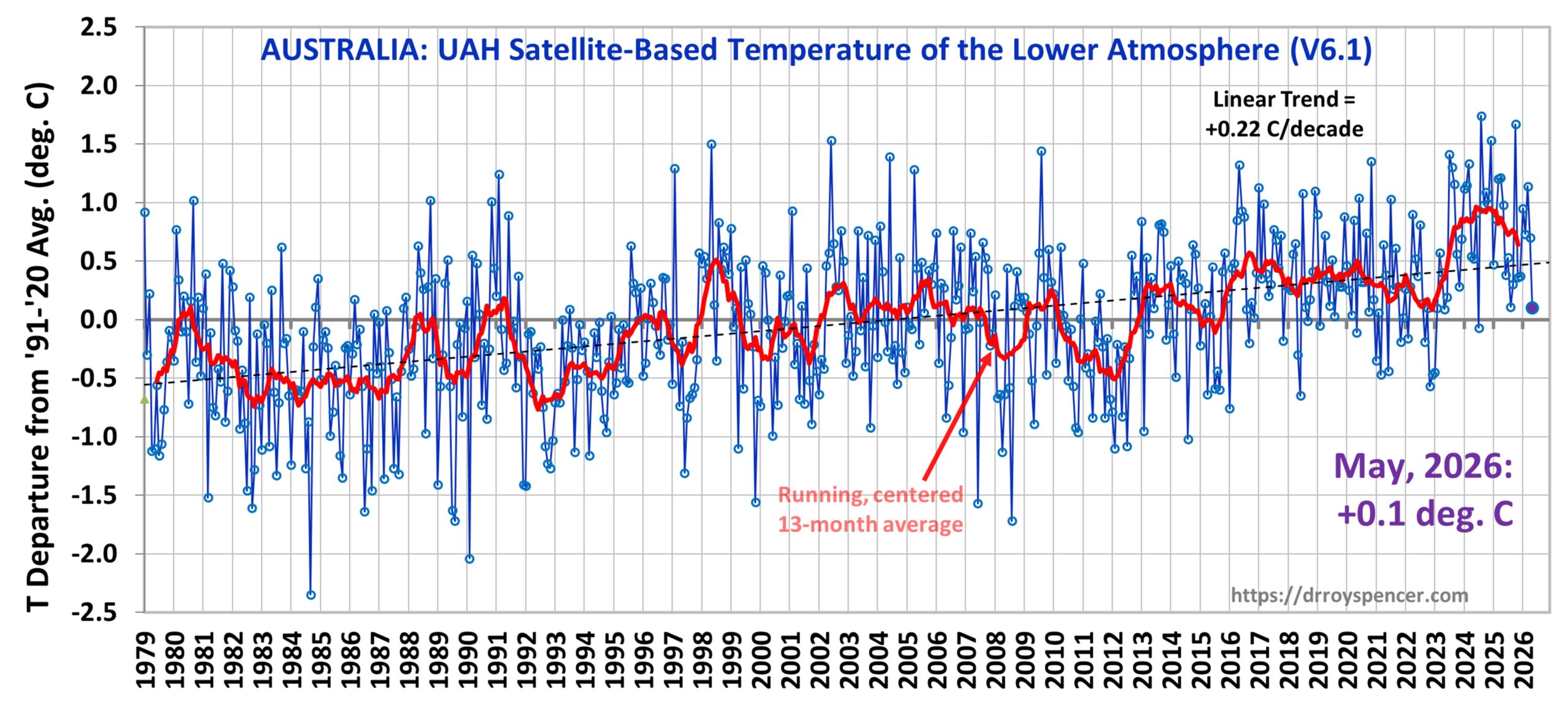
Time Series Plots for Tropics, USA48, Canada, and Australia
The full UAH Global Temperature Report, along with the LT global gridpoint anomaly map for September, 2026 and a more detailed analysis by John Christy, should be available within the next several days here.
The monthly anomalies for various regions for the four deep layers we monitor from satellites will be available in the next several days at the following locations:
The Version 6.1 global average lower tropospheric temperature (LT) anomaly for August, 2026 was +0.68 deg. C departure from the 1991-2020 mean, up from the July, 2026 value of +0.48 deg. C. It appears the effects of the strengthening major El Nino event are beginning to appear in the global average tropospheric temperature, with an August temperature anomaly of +0.9 deg. C in the tropics. This month I’ve added a plot of tropical temperatures (below).
The Version 6.1 global area-averaged linear temperature trend (January 1979 through August 2026) remains at +0.16 deg/ C/decade (+0.22 C/decade over land, +0.13 C/decade over oceans).
The following table lists various regional Version 6.1 LT departures from the 30-year (1991-2020) average for the last 32 months (record highs are in red).
Year
Mon
Globe
NHem
SHem
Tropic
US48
Arctic
Aust.
Can.
2024
Jan
+0.80
+1.02
+0.57
+1.20
-0.19
+0.40
+1.12
+0.97
2024
Feb
+0.88
+0.94
+0.81
+1.16
+1.31
+0.85
+1.16
+2.45
2024
Mar
+0.88
+0.96
+0.80
+1.25
+0.22
+1.05
+1.34
+1.12
2024
Apr
+0.94
+1.12
+0.76
+1.15
+0.86
+0.88
+0.54
+1.39
2024
May
+0.77
+0.77
+0.78
+1.20
+0.04
+0.20
+0.52
+0.67
2024
June
+0.69
+0.78
+0.60
+0.85
+1.36
+0.63
+0.91
+0.19
2024
July
+0.73
+0.86
+0.61
+0.96
+0.44
+0.56
-0.07
+1.15
2024
Aug
+0.75
+0.81
+0.69
+0.74
+0.40
+0.88
+1.75
+1.36
2024
Sep
+0.81
+1.04
+0.58
+0.82
+1.31
+1.48
+0.98
2024
Oct
+0.75
+0.89
+0.60
+0.63
+1.89
+0.81
+1.09
+0.89
2024
Nov
+0.64
+0.87
+0.40
+0.53
+1.11
+0.79
+1.00
+1.61
2024
Dec
+0.61
+0.75
+0.47
+0.52
+1.41
+1.12
+1.54
+1.65
2025
Jan
+0.45
+0.70
+0.21
+0.24
-1.07
+0.74
+0.48
+1.04
2025
Feb
+0.50
+0.55
+0.45
+0.26
+1.03
+2.10
+0.87
-0.35
2025
Mar
+0.57
+0.73
+0.41
+0.40
+1.24
+1.23
+1.20
+0.80
2025
Apr
+0.61
+0.76
+0.46
+0.36
+0.81
+0.85
+1.21
+0.45
2025
May
+0.50
+0.45
+0.55
+0.30
+0.15
+0.75
+0.98
+0.81
2025
June
+0.48
+0.48
+0.47
+0.30
+0.80
+0.05
+0.39
-0.22
2025
July
+0.36
+0.49
+0.23
+0.45
+0.32
+0.40
+0.53
-0.23
2025
Aug
+0.39
+0.39
+0.39
+0.16
-0.06
+0.82
+0.11
+0.62
2025
Sep
+0.53
+0.56
+0.49
+0.35
+0.38
+0.77
+0.30
+2.44
2025
Oct
+0.53
+0.52
+0.55
+0.24
+1.12
+1.42
+1.67
+2.59
2025
Nov
+0.43
+0.59
+0.27
+0.24
+1.32
+0.78
+0.36
+1.47
2025
Dec
+0.30
+0.45
+0.15
+0.19
+2.10
+0.32
+0.37
-1.86
2026
Jan
+0.35
+0.51
+0.19
+0.09
+0.30
+1.40
+0.95
+1.17
2026
Feb
+0.39
+0.54
+0.23
+0.03
+1.91
-0.48
+0.73
+0.32
2026
Mar
+0.38
+0.33
+0.42
+0.07
+3.74
-0.48
+1.14
-3.17
2026
Apr
+0.39
+0.43
+0.34
+0.23
+1.20
+0.30
+0.70
-0.89
2026
May
+0.53
+0.46
+0.60
+0.58
+0.21
+0.34
+0.10
+0.21
2026
June
+0.46
+0.54
+0.38
+0.57
+0.64
+1.01
+0.38
+0.99
2026
July
+0.48
+0.68
+0.27
+0.85
+1.14
+0.53
-0.22
+0.78
2026
August
+0.68
+0.76
+0.59
+0.90
+0.60
+0.80
+0.39
+0.71
Year
Mon
Globe
NHem
SHem
Tropic
US48
Arctic
Aust.
Can.
Time Series Plots for Tropics, USA48, Canada, and Australia
The full UAH Global Temperature Report, along with the LT global gridpoint anomaly map for August, 2026 and a more detailed analysis by John Christy, should be available within the next several days here. John officially retired with emeritus professor status on July 1, 2026, and is now working as a part-time employee of UAH.
The monthly anomalies for various regions for the four deep layers we monitor from satellites will be available in the next several days at the following locations:
Recent photo of Lake Mead behind Hoover Dam (Newsweek).
NOTE: I’ve made a couple of updates/clarifications below based upon comments on this post.
Lake Mead behind Hoover Dam is now within several feet of the lowest level at which turbine power generation must be greatly curtailed. Recent news articles often blame the cause on a “millennium drought” being experienced in the West. Of course, much of the western U.S. experiences drought conditions every summer, which is part of the normal climate there. Tens of millions of people like to live where it is sunny most of the year, and agriculture thrives where photosynthesis (lots of sunshine) is abundant… assuming enough water supply for irrigation.
Obviously, people need water, which is why virtually no one lives in the Sahara Desert. Add in the beauty of the Pacific Ocean, and it was inevitable that water demand would exceed supply. Even in 1922, before most people moved out west, the Colorado River Compact was negotiated to divide up the Colorado River’s water among seven southwestern states: California, Nevada, New Mexico, Arizona, Colorado, Utah, and Wyoming.
Most of the water in the Colorado River is from snowmelt in the Rocky Mountains. Most (50% to 70%) goes to agriculture. And, yes, the annual runoff flows into Lake Mead (which was filled after construction of Hoover Dam was mostly completed in 1935) have been below “normal” in recent years. But calling recent reduced streamflow (and as a result, lower Lake Mead water levels) the result of a “millennium drought” is sloppy reporting.
Numerous studies suggest that the original Colorado River Compact of 1922 was based upon a period of unusually high precipitation. This was discussed in a paper entitled “New Streamflow Reconstructions for the Upper Colorado River Basin: Placing Recent Droughts into a Centuries-Long Context“, which is a very readable review of various studies that have reconstructed Colorado River flows at Lee Ferry over the last 500 years from tree ring data. While the paper is a little dated (2006), the conclusions remain the same today.
Here are a couple of noteworthy quotes from that paper (bold added):
“The Stockton and Jacoby reconstruction of the annual flows from 1520 to 1961 contained several important findings, including that the highest sustained flows in the entire record occurred in the first part of the 20th century, the period upon which the Colorado River Compact of 1922 was negotiated, while the most persistent and severe drought occurred in the late 16th century.“
“…Colorado River allocations were based on one of the wettest periods in the past five centuries, while droughts more severe than any 20th-21st century event have occurred in the past.”
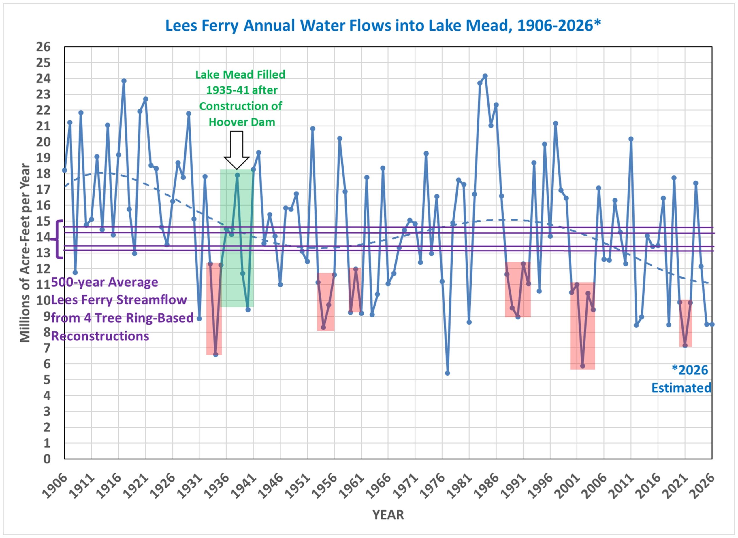
I’ve created a chart of the annual streamflows at Lee Ferry with some annotations showing periods of 3+ year droughts, the long-term trend (5th order polynomial fit) since stream gage data started in 1906, and four different estimates of the long-term (500-year) normal streamflow at Lee Ferry reconstructed from tree ring data.(UPDATE: the 2026 estimate is not just a repeat of the 2025 measurement, it is the central estimate of several quantitative evaluations of what the 2026 water year [October through September] will be based upon Lee Ferry gage measurements.)
As can be seen, the period before Hoover Dam was constructed was unusually wet. From the 1930s onward, there has been little net trend with some very wet years and very dry years, with up to a factor of 4-to-5 variations in the annual flows into Lake Mead. Six drought periods of at least 3 consecutive years are shown in red. Note that it took only 5 years to completely fill Lake Mead, which was accomplished by reducing the streamflow below the dam by about 30% to 40% of what the normal flows have been in recent decades.
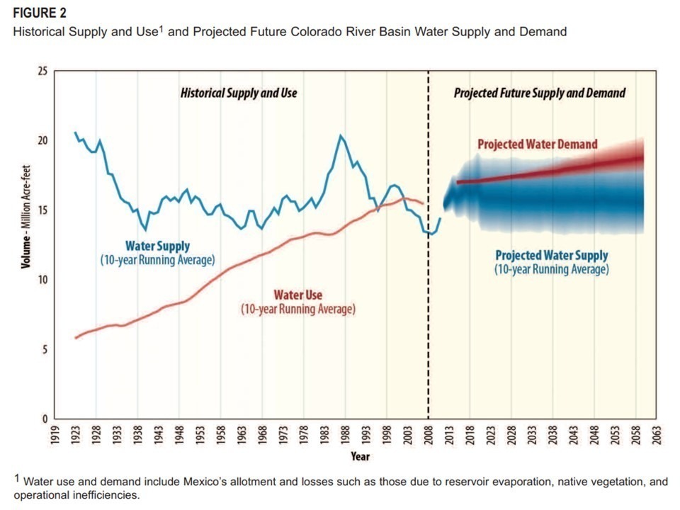
From the above graph, I think one would be hard pressed to say there has been a statistically significant decrease in streamflow since the 1930s. (UPDATE: the linear trend for 1932 [a wet year] to 2025 is -0.013 +/- 0.016 million acre-feet per year, so it is not significant at the 68% confidence level). The major problem is that water usage exceeds what Mother Nature can reliably provide on a long-term basis. Several years ago I discussed this problem in a post in which I included the following graph (also rather dated) of Colorado River water supply versus usage.
As can be seen, since about 2000, usage has exceeded supply, and given the natural multi-year variations in streamflow, it was only a matter of time before Lake Mead water levels would fall to operationally low levels.
In that same post I showed the average of over 100 CMIP6 climate model runs that show precipitation in the Colorado River watershed increasing substantially with global warming, so blaming the recent dry years on human-caused climate change seems a stretch. (UPDATE: While it is true that drought is a function of both precipitation and evaporation, and warming can cause drought even if precipitation does not change, water releases from Hoover Dam have been declining since 1998, so increased evapotranspiration from irrigation uses downstream of the dam [the main use of Colorado River water] cannot explain decreasing Lake Mead water levels. Direct evaporation from the lake surface is very small and changes little with warming. And there has been no statistically significant trend in streamflow input at Lee Ferry since 1932.)
And calling the recent dry years a “millennium drought” is just fake news
The Version 6.1 global average lower tropospheric temperature (LT) anomaly for July, 2026 was +0.48 deg. C departure from the 1991-2020 mean, which is statistically unchanged from the June, 2026 value of +0.46 deg. C.
The Version 6.1 global area-averaged linear temperature trend (January 1979 through July 2026) remains at +0.16 deg/ C/decade (+0.22 C/decade over land, +0.13 C/decade over oceans).
The following table lists various regional Version 6.1 LT departures from the 30-year (1991-2020) average for the last 31 months (record highs are in red).
Year
Mon
Globe
NHem
SHem
Tropic
US48
Arctic
Aust.
Can.
2024
Jan
+0.80
+1.02
+0.57
+1.20
-0.19
+0.40
+1.12
+0.97
2024
Feb
+0.88
+0.94
+0.81
+1.16
+1.31
+0.85
+1.16
+2.45
2024
Mar
+0.88
+0.96
+0.80
+1.25
+0.22
+1.05
+1.34
+1.12
2024
Apr
+0.94
+1.12
+0.76
+1.15
+0.86
+0.88
+0.54
+1.39
2024
May
+0.77
+0.77
+0.78
+1.20
+0.04
+0.20
+0.52
+0.67
2024
June
+0.69
+0.78
+0.60
+0.85
+1.36
+0.63
+0.91
+0.19
2024
July
+0.73
+0.86
+0.61
+0.96
+0.44
+0.56
-0.07
+1.15
2024
Aug
+0.75
+0.81
+0.69
+0.74
+0.40
+0.88
+1.75
+1.36
2024
Sep
+0.81
+1.04
+0.58
+0.82
+1.31
+1.48
+0.98
2024
Oct
+0.75
+0.89
+0.60
+0.63
+1.89
+0.81
+1.09
+0.89
2024
Nov
+0.64
+0.87
+0.40
+0.53
+1.11
+0.79
+1.00
+1.61
2024
Dec
+0.61
+0.75
+0.47
+0.52
+1.41
+1.12
+1.54
+1.65
2025
Jan
+0.45
+0.70
+0.21
+0.24
-1.07
+0.74
+0.48
+1.04
2025
Feb
+0.50
+0.55
+0.45
+0.26
+1.03
+2.10
+0.87
-0.35
2025
Mar
+0.57
+0.73
+0.41
+0.40
+1.24
+1.23
+1.20
+0.80
2025
Apr
+0.61
+0.76
+0.46
+0.36
+0.81
+0.85
+1.21
+0.45
2025
May
+0.50
+0.45
+0.55
+0.30
+0.15
+0.75
+0.98
+0.81
2025
June
+0.48
+0.48
+0.47
+0.30
+0.80
+0.05
+0.39
-0.22
2025
July
+0.36
+0.49
+0.23
+0.45
+0.32
+0.40
+0.53
-0.23
2025
Aug
+0.39
+0.39
+0.39
+0.16
-0.06
+0.82
+0.11
+0.62
2025
Sep
+0.53
+0.56
+0.49
+0.35
+0.38
+0.77
+0.30
+2.44
2025
Oct
+0.53
+0.52
+0.55
+0.24
+1.12
+1.42
+1.67
+2.59
2025
Nov
+0.43
+0.59
+0.27
+0.24
+1.32
+0.78
+0.36
+1.47
2025
Dec
+0.30
+0.45
+0.15
+0.19
+2.10
+0.32
+0.37
-1.86
2026
Jan
+0.35
+0.51
+0.19
+0.09
+0.30
+1.40
+0.95
+1.17
2026
Feb
+0.39
+0.54
+0.23
+0.03
+1.91
-0.48
+0.73
+0.32
2026
Mar
+0.38
+0.33
+0.42
+0.07
+3.74
-0.48
+1.14
-3.17
2026
Apr
+0.39
+0.43
+0.34
+0.23
+1.20
+0.30
+0.70
-0.89
2026
May
+0.53
+0.46
+0.60
+0.58
+0.21
+0.34
+0.10
+0.21
2026
June
+0.46
+0.54
+0.38
+0.57
+0.64
+1.01
+0.38
+0.99
2026
July
+0.48
+0.68
+0.27
+0.85
+1.14
+0.53
-0.22
+0.78
Year
Mon
Globe
NHem
SHem
Tropic
US48
Arctic
Aust.
Can.
Time Series Plots for USA48, Canada, and Australia
The full UAH Global Temperature Report, along with the LT global gridpoint anomaly map for July, 2026 and a more detailed analysis by John Christy, should be available within the next several days here. John officially retired on July 1, 2026, but will continue working as a part-time employee of UAH.
The monthly anomalies for various regions for the four deep layers we monitor from satellites will be available in the next several days at the following locations:
The Version 6.1 global average lower tropospheric temperature (LT) anomaly for June, 2026 was +0.46 deg. C departure from the 1991-2020 mean, which is down from the May, 2026 value of +0.53 deg. C.
The Version 6.1 global area-averaged linear temperature trend (January 1979 through June 2026) remains at +0.16 deg/ C/decade (+0.22 C/decade over land, +0.13 C/decade over oceans).
The following table lists various regional Version 6.1 LT departures from the 30-year (1991-2020) average for the last 30 months (record highs are in red).
Year
Mon
Globe
NHem
SHem
Tropic
US48
Arctic
Aust.
Can.
2024
Jan
+0.80
+1.02
+0.57
+1.20
-0.19
+0.40
+1.12
+0.97
2024
Feb
+0.88
+0.94
+0.81
+1.16
+1.31
+0.85
+1.16
+2.45
2024
Mar
+0.88
+0.96
+0.80
+1.25
+0.22
+1.05
+1.34
+1.12
2024
Apr
+0.94
+1.12
+0.76
+1.15
+0.86
+0.88
+0.54
+1.39
2024
May
+0.77
+0.77
+0.78
+1.20
+0.04
+0.20
+0.52
+0.67
2024
June
+0.69
+0.78
+0.60
+0.85
+1.36
+0.63
+0.91
+0.19
2024
July
+0.73
+0.86
+0.61
+0.96
+0.44
+0.56
-0.07
+1.15
2024
Aug
+0.75
+0.81
+0.69
+0.74
+0.40
+0.88
+1.75
+1.36
2024
Sep
+0.81
+1.04
+0.58
+0.82
+1.31
+1.48
+0.98
2024
Oct
+0.75
+0.89
+0.60
+0.63
+1.89
+0.81
+1.09
+0.89
2024
Nov
+0.64
+0.87
+0.40
+0.53
+1.11
+0.79
+1.00
+1.61
2024
Dec
+0.61
+0.75
+0.47
+0.52
+1.41
+1.12
+1.54
+1.65
2025
Jan
+0.45
+0.70
+0.21
+0.24
-1.07
+0.74
+0.48
+1.04
2025
Feb
+0.50
+0.55
+0.45
+0.26
+1.03
+2.10
+0.87
-0.35
2025
Mar
+0.57
+0.73
+0.41
+0.40
+1.24
+1.23
+1.20
+0.80
2025
Apr
+0.61
+0.76
+0.46
+0.36
+0.81
+0.85
+1.21
+0.45
2025
May
+0.50
+0.45
+0.55
+0.30
+0.15
+0.75
+0.98
+0.81
2025
June
+0.48
+0.48
+0.47
+0.30
+0.80
+0.05
+0.39
-0.22
2025
July
+0.36
+0.49
+0.23
+0.45
+0.32
+0.40
+0.53
-0.23
2025
Aug
+0.39
+0.39
+0.39
+0.16
-0.06
+0.82
+0.11
+0.62
2025
Sep
+0.53
+0.56
+0.49
+0.35
+0.38
+0.77
+0.30
+2.44
2025
Oct
+0.53
+0.52
+0.55
+0.24
+1.12
+1.42
+1.67
+2.59
2025
Nov
+0.43
+0.59
+0.27
+0.24
+1.32
+0.78
+0.36
+1.47
2025
Dec
+0.30
+0.45
+0.15
+0.19
+2.10
+0.32
+0.37
-1.86
2026
Jan
+0.35
+0.51
+0.19
+0.09
+0.30
+1.40
+0.95
+1.17
2026
Feb
+0.39
+0.54
+0.23
+0.03
+1.91
-0.48
+0.73
+0.32
2026
Mar
+0.38
+0.33
+0.42
+0.07
+3.74
-0.48
+1.14
-3.17
2026
Apr
+0.39
+0.43
+0.34
+0.23
+1.20
+0.30
+0.70
-0.89
2026
May
+0.53
+0.46
+0.60
+0.58
+0.21
+0.34
+0.10
+0.21
2026
June
+0.46
+0.54
+0.38
+0.57
+0.64
+1.01
+0.38
+0.99
Year
Mon
Globe
NHem
SHem
Tropic
US48
Arctic
Aust.
Can.
Time Series Plots for USA48, Canada, and Australia
The full UAH Global Temperature Report, along with the LT global gridpoint anomaly map for June, 2026 and a more detailed analysis by John Christy, should be available within the next several days here. John officially retired yesterday, July 1, 2026, but will continue working as a part-time employee of UAH.
The monthly anomalies for various regions for the four deep layers we monitor from satellites will be available in the next several days at the following locations:
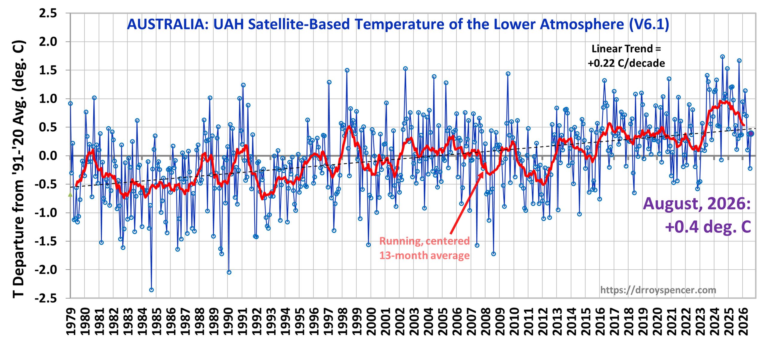
This month I’m adding Australia to the Global, USA48, and Canada time series plots.
The Version 6.1 global average lower tropospheric temperature (LT) anomaly for May, 2026 was +0.53 deg. C departure from the 1991-2020 mean, which is up from the April, 2026 value of +0.39 deg. C..
The Version 6.1 global area-averaged linear temperature trend (January 1979 through May 2026) remains at +0.16 deg/ C/decade (+0.22 C/decade over land, +0.13 C/decade over oceans).
A Note on These Tropospheric Temperature Anomalies vs. Surface Temperature Anomalies
It has been a while since I have discussed the main reason why our global monthly satellite-based tropospheric temperature anomalies can sometimes differ by quite a lot from the global monthly surface temperature anomalies. A good example is the last 2 months. In April, our +0.39 deg. C anomaly was statistically identical to the +0.38 deg. C surface temperature anomaly from the NOAA Climate Data Assimilation System (CDAS, which I take from WeatherBell.com maps). But then last month (May) the CDAS anomaly went down slightly (+ 0.34 deg. C), while our UAH anomaly went up considerably (+0.53 deg. C). These month-to-month fluctuations in the relationship between surface and tropospheric temperature changes are almost certainly dominated by fluctuations in moist convective heat transfer from the surface to the free troposphere. When there is a burst of extra convection (usually in the tropics), it cools the surface and warms the free troposphere more than normal, which is probably what happened last month (May).
The following table lists various regional Version 6.1 LT departures from the 30-year (1991-2020) average for the last 29 months (record highs are in red).
Year
Mon
Globe
NHem
SHem
Tropic
US48
Arctic
Aust.
Can.
2024
Jan
+0.80
+1.02
+0.57
+1.20
-0.19
+0.40
+1.12
+0.97
2024
Feb
+0.88
+0.94
+0.81
+1.16
+1.31
+0.85
+1.16
+2.45
2024
Mar
+0.88
+0.96
+0.80
+1.25
+0.22
+1.05
+1.34
+1.12
2024
Apr
+0.94
+1.12
+0.76
+1.15
+0.86
+0.88
+0.54
+1.39
2024
May
+0.77
+0.77
+0.78
+1.20
+0.04
+0.20
+0.52
+0.67
2024
June
+0.69
+0.78
+0.60
+0.85
+1.36
+0.63
+0.91
+0.19
2024
July
+0.73
+0.86
+0.61
+0.96
+0.44
+0.56
-0.07
+1.15
2024
Aug
+0.75
+0.81
+0.69
+0.74
+0.40
+0.88
+1.75
+1.36
2024
Sep
+0.81
+1.04
+0.58
+0.82
+1.31
+1.48
+0.98
2024
Oct
+0.75
+0.89
+0.60
+0.63
+1.89
+0.81
+1.09
+0.89
2024
Nov
+0.64
+0.87
+0.40
+0.53
+1.11
+0.79
+1.00
+1.61
2024
Dec
+0.61
+0.75
+0.47
+0.52
+1.41
+1.12
+1.54
+1.65
2025
Jan
+0.45
+0.70
+0.21
+0.24
-1.07
+0.74
+0.48
+1.04
2025
Feb
+0.50
+0.55
+0.45
+0.26
+1.03
+2.10
+0.87
-0.35
2025
Mar
+0.57
+0.73
+0.41
+0.40
+1.24
+1.23
+1.20
+0.80
2025
Apr
+0.61
+0.76
+0.46
+0.36
+0.81
+0.85
+1.21
+0.45
2025
May
+0.50
+0.45
+0.55
+0.30
+0.15
+0.75
+0.98
+0.81
2025
June
+0.48
+0.48
+0.47
+0.30
+0.80
+0.05
+0.39
-0.22
2025
July
+0.36
+0.49
+0.23
+0.45
+0.32
+0.40
+0.53
-0.23
2025
Aug
+0.39
+0.39
+0.39
+0.16
-0.06
+0.82
+0.11
+0.62
2025
Sep
+0.53
+0.56
+0.49
+0.35
+0.38
+0.77
+0.30
+2.44
2025
Oct
+0.53
+0.52
+0.55
+0.24
+1.12
+1.42
+1.67
+2.59
2025
Nov
+0.43
+0.59
+0.27
+0.24
+1.32
+0.78
+0.36
+1.47
2025
Dec
+0.30
+0.45
+0.15
+0.19
+2.10
+0.32
+0.37
-1.86
2026
Jan
+0.35
+0.51
+0.19
+0.09
+0.30
+1.40
+0.95
+1.17
2026
Feb
+0.39
+0.54
+0.23
+0.03
+1.91
-0.48
+0.73
+0.32
2026
Mar
+0.38
+0.33
+0.42
+0.07
+3.74
-0.48
+1.14
-3.17
2026
Apr
+0.39
+0.43
+0.34
+0.23
+1.20
+0.30
+0.70
-0.89
2026
May
+0.53
+0.53
+0.53
+0.58
+0.21
+0.33
+0.10
+0.21
Year
Mon
Globe
NHem
SHem
Tropic
US48
Arctic
Aust.
Can.
Time Series Plots for USA48, Canada, and Australia
The full UAH Global Temperature Report, along with the LT global gridpoint anomaly map for May, 2026 and a more detailed analysis by John Christy, should be available within the next several days here.
The monthly anomalies for various regions for the four deep layers we monitor from satellites will be available in the next several days at the following locations:
There was a recent weeks-long exchange of emails between many climate people — professional and amateur — regarding the idea that air pressure (in combination with absorbed solar energy) is what causes temperature. There were insults launched at those who refused to believe what a certain physics-trained person says should be a revolution in our understanding of planetary temperatures. That person even managed to get a paper published in a journal that (in my opinion) used reviewers who were in over their heads on the subject.
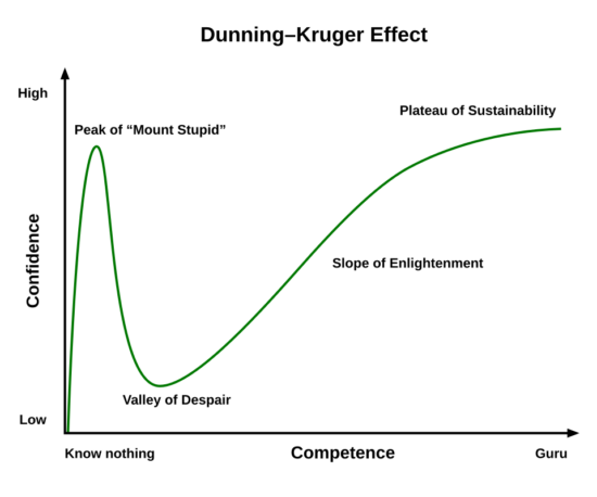
The whole ordeal makes me think of the Dunning-Kruger Effect, which is the tendency for people who start to understand a complex subject to overestimate their level of understanding. This then leads to a point of peak overconfidence (climbing “Mount Stupid”), which then gradually relaxes as more is learned and the person increasingly realizes that the subject is more complicated and nuanced than they originally thought.
I claim that the person in question who thinks [pressure + absorbed solar energy = temperature] is still stuck on Mount Stupid.
The reason I bring this up again (I’ve preached on it before) is that many have been misled into believing the “theory”. As a result, I have spent many years responding to questions from the public (including science-savvy citizens) regarding the issue. Many have been convinced by the “theory”, and have joined the proponent of the theory on Mount Stupid.
After lurking in the weeks-long email discussion, I finally responded with the following summary of the issue. I have removed the person’s name to protect the not-so-innocent.
SUBJECT: Where <NAME REDACTED> Is Right… and Where <PRONOUN REDACTED> Is Wrong
All:
After working in meteorology and then climate during my 40+ year career, I think I can offer some insight into the issues being discussed in these emails. Like <NAME REDACTED>, I have always been skeptical of what I have been told until I could fully understand an issue for myself.
I’m sure the following explanations will be of help to many of you. (I suspect <NAME REDACTED> is too invested in theories to change <PRONOUN REDACTED> mind.) Many of the concepts are not trivial, and I will admit it wasn’t until many years after all of my education (PhD Meteorology) that I finally understood a few of them, because they were not taught in school. Dick Lindzen helped me in this in the early climate research years.
Most of what follows is fundamental atmospheric thermodynamics, and I question whether <NAME REDACTED> really did take a university-level Atmospheric Thermodynamics course. If he did, I’d like to know where.
And if <PRONOUN REDACTED> shows me <PRONOUN REDACTED> grades, I’ll show <PRONOUN REDACTED> mine.
A THOUGHT EXPERIMENT
Imagine you could suddenly dump an extra 1 atmosphere of air on top of the existing atmosphere, what would happen to air temperature in the 1 ATM below? Just as <NAME REDACTED> would predict, the temperature of the original atmosphere below would increase greatly through adiabatic compression.
But what would happen NEXT?….
The high [hot] atmospheric temperatures in the lower atmosphere would then be far out of energy balance compared to what existed before. The result would be cooling of all of that air that was heated through adiabatic (or nearly so) compression (work done on the lower atmosphere) until a new state of energy equilibrium was reached. The energy loss would be through infrared radiation of the hotter air.
In fact is it always ENERGY BALANCE that determines temperature, through the 1st Law of Thermodynamics. A change in temperature is proportional to the rate of energy input minus the energy output (which includes any work done in the process).
In contrast, the Ideal Gas Law (PV=nRT) cannot tell you what the temperature “should be”. It only says how the variables P, V, and T are interrelated during the process of re-equilibration and in the final equilibrium state. What <NAME REDACTED> misses in <PRONOUN REDACTED> theory is the “n” part of the equation (the number of moles, or mass… which is in the density form of the equation, P = rho RT). In my hypothetical 2-atmosphere thought experiment, as the lower atmosphere cools to reach a new state of energy equilibrium with the solar input, the decreasing temperature causes an increase in the air density (“shrinkage”), and the pressure remains the same… even while the temperature is changing.
Specifically, following the 1st Law, the internal temperature of a volume of atmosphere exposed to an energy INPUT will increase until the temperature-dependent energy OUTPUT processes equal the rate of energy gain. This is true of every physical system… the atmosphere, a pot of water on the stove, a car’s engine, the human body, the interior of the sun, etc. That energy equilibrium is what determines the final temperature. (In the real atmosphere, there are constant energy imbalances and thus changes in temperature; Trenberth’s global-average energy balance diagram is only useful to gain a conceptual understanding of the relative role of the major energy flows in the global-average climate system.)
THE IDEAL GAS LAW
Again, the Ideal Gas Law equation (PV=nRT) cannot tell you what the temperature of a gas should be, only energy flows in and out can do that. The gas law just tells you how the P, n, and T are interrelated for a given volume (V) of air. Yes, <NAME REDACTED>, on short time scales, ascending air cools and descending air warms, but if all of that motion was to stop, energy flow processes would then determine what the final temperature would be… not what the air pressure is.
For a given surface air pressure, a huge range of temperatures is possible, and that huge range is all due to energy flow processes. Again, if the near-surface air temperature over the whole planet is much higher than local energy flow processes can support, the temperature falls, and the air’s volume shrinks (or density, rho, increases, according to the equivalent Ideal Gas Law equation, P=rhoRT). The surface air pressure remains the same because the total mass of the atmosphere is unchanged.
SO WHY MIGHT THERE BE A CLOSE RELATIONSHIP BETWEEN DIFFERENT PLANET’S LOWER ATMOSPHERIC TEMPERATURE AND PRESSURE?
I haven’t studied the atmospheres of other planets, because I don’t care. Even if those other planets did not exist, they are not necessary for understanding our own atmosphere. But if indeed <NAME REDACTED> is correct about a close statistical relationship between different planets’ surface air pressure and temperature, after adjusting for solar input, then I suspect it’s because the more atmosphere there is, the more greenhouse gases there are.
On the subject of GHGs, I’ve forgotten… does <NAME REDACTED> believe that air absorbs and emits IR energy? Because the greenhouse effect is a necessary consequence of that absorption/emission. Energetically, the GHE is a radiative insulator. It’s analogous to adding insulation to a heated building’s walls in winter. For a given energy input into the building, the air temperature inside will rise, and the outside of the walls will experience a temperature fall. This is exactly what the GHE does to the atmospheric temperature profile (in an energetic sense.. clearly involving radiation rather than conduction as a heat transfer mechanism).
If <NAME REDACTED> doesn’t believe air absorbs IR energy, how does <PRONOUN REDACTED> explain all of the thousands of spectroscopic measurements of CO2, water vapor, and methane as a function of temperature and pressure? And if <PRONOUN REDACTED> does believe the atmosphere absorbs and emits IR energy, then <PRONOUN REDACTED> must also believe in a greenhouse effect, because it is a necessary consequence…. the greenhouse effect in planetary atmospheres always causes warming of the lower atmosphere and cooling of the upper atmosphere.
(BTW, it is a common misconception that air which absorbs IR energy immediately loses that energy through emission of IR. Not true. Look up the “kinetic theory of gases” and related concepts. When CO2 or H2O vapor molecules absorb IR photons they extremely rapidly lose their extra energy to other air molecules through collisions. This happens much faster [by a factor of ~50,000] than the time it takes to re-emit energy through IR photons. This is how IR absorption immediately leads to “thermalization” [a term I hate].
Furthermore, it is crucial to understand that since IR absorption is largely independent of temperature, but IR loss is VERY dependent upon temperature, almost all air in the atmosphere is in a continual state of IR energy imbalance. Much of that imbalance is what [is balanced by] convective overturning.
WHAT IS THE ROLE OF THE ADIABATIC LAPSE RATE?
The adiabatic lapse rate in the troposphere (9.8 deg C per km without moisture condensation) is the RESULT OF convective overturning. If condensation of moisture is involved in updrafts, then the lapse rate is lower. Like the Ideal Gas Law, it doesn’t tell you what the temperature “should” be. It just tells you how the temperature of an air parcel changes during ascent or descent, if there is no energy gain or loss (“a-diabatic”). [But there are energy gains and losses occurring everywhere, all the time, and those determine what the absolute temperature will be — not pressure.]
HOW DOES THE GREENHOUSE EFFECT PLAY INTO THE LAPSE RATE?
This is a very interesting subject. It is something that even many atmospheric scientists and climate researchers don’t really understand. The combination of solar heating of the surface and IR absorption and emission by the surface and atmosphere ALONE, WITHOUT ANY CONVECTIVE OVERTURNING would result in an extremely steep tropospheric lapse rate, with very high surface temperatures and exceedingly cold upper tropospheric temperatures. This was first demonstrated by Manabe & Strickler (1964), and it’s called the “pure radiative equilibrium” case. It is sort of what makes the term “greenhouse effect” technically correct; like a real greenhouse inhibiting convective heat loss [because it has a roof], the greenhouse effect is, by definition, what happens WITHOUT the resulting convective overturning.
But in the real world, convective overturning is the RESPONSE to this GHE destabilization! So, that 33 deg. GHE warming people talk about? That’s not the GHE. It’s the GHE + CONVECTION. Without convection, that 33 deg. C figure would be more like 65 or 75 deg. C. Which then leads to another fascinating question…
WHAT WOULD HAPPEN IF THE ATMOSPHERE DID NOT ABSORB AND EMIT IR ENERGY?
Imagine a cold planetary atmosphere with no energy input. Then, turn on the sun. Solar heating of the surface would warm the atmosphere through convective overturning. But the [deep] atmosphere would have no way to shed that energy to cool in the presence of all of that energy input. The temperature of the [deep] atmosphere would then continue to rise until it had the same temperature as the surface, through its entire depth. Long before that process finished convective overturning would have stopped, because the atmosphere would be too stable to support convection. The atmosphere would eventually become isothermal (or nearly so, since there might be some planetary scale overturning between the tropics and the poles, due to their different rates of solar input), with the same temperature as the surface. Interestingly, as a result all weather activity would cease. All clouds would probably disappear, resulting in higher temperatures. Any [remaining] circulation systems would have a planetary scale, because the horizontal scale of those systems are related to the lapse rate (through the “Rossby radius of deformation”), which is also why the stratosphere only has planetary-scale circulations.
This month I’m adding plots for USA48 and Canada, too.
The Version 6.1 global average lower tropospheric temperature (LT) anomaly for April, 2026 was +0.39 deg. C departure from the 1991-2020 mean, which remains statistically unchanged for 4 months now.
The Version 6.1 global area-averaged linear temperature trend (January 1979 through April 2026) remains at +0.16 deg/ C/decade (+0.22 C/decade over land, +0.13 C/decade over oceans).
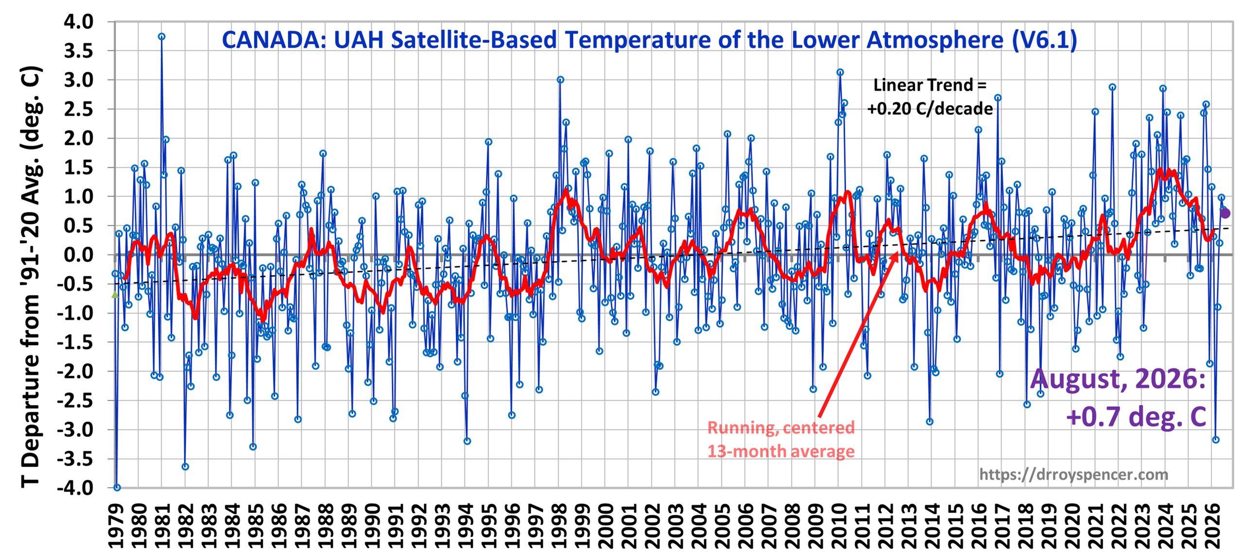
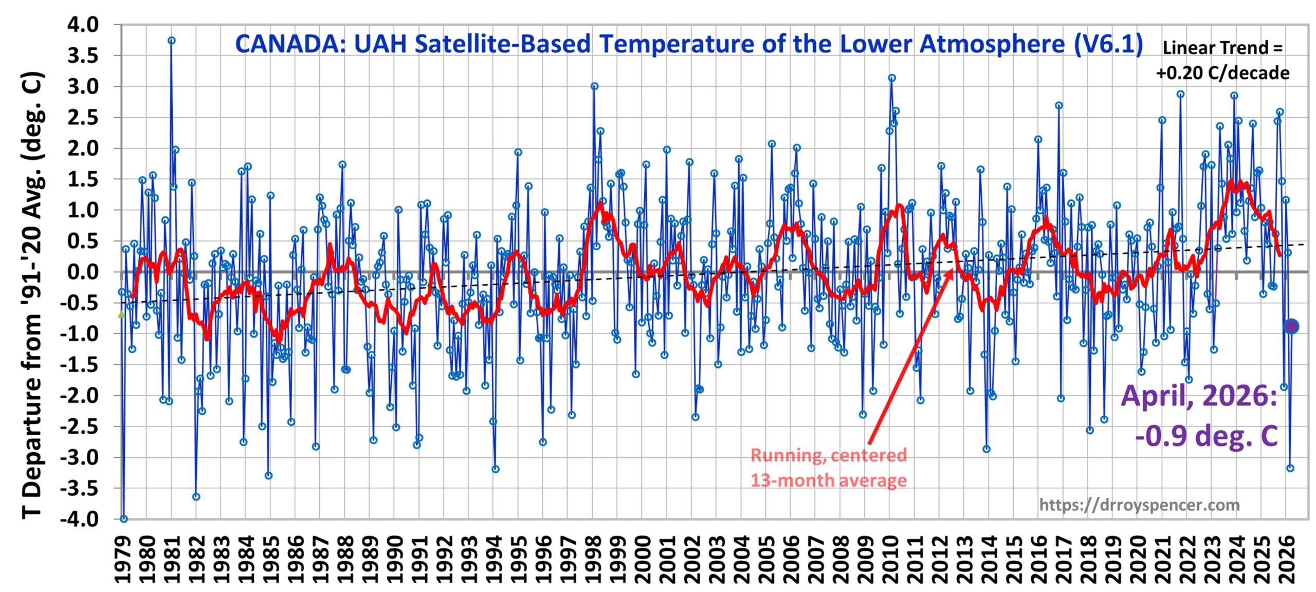
The following table lists various regional Version 6.1 LT departures from the 30-year (1991-2020) average for the last 28 months (record highs are in red). Note I’ve added Canada to the table this month, by request (although WordPress won’t allow me to add September 2024 for some reason). The warmest April in Canada was in 2010 (+2.61 deg. C), while the warmest anomaly out of all months was in January 1981 (+3.75 deg. C).
Year
Mon
Globe
NHem
SHem
Tropic
US48
Arctic
Aust.
Can.
2024
Jan
+0.80
+1.02
+0.57
+1.20
-0.19
+0.40
+1.12
+0.97
2024
Feb
+0.88
+0.94
+0.81
+1.16
+1.31
+0.85
+1.16
+2.45
2024
Mar
+0.88
+0.96
+0.80
+1.25
+0.22
+1.05
+1.34
+1.12
2024
Apr
+0.94
+1.12
+0.76
+1.15
+0.86
+0.88
+0.54
+1.39
2024
May
+0.77
+0.77
+0.78
+1.20
+0.04
+0.20
+0.52
+0.67
2024
June
+0.69
+0.78
+0.60
+0.85
+1.36
+0.63
+0.91
+0.19
2024
July
+0.73
+0.86
+0.61
+0.96
+0.44
+0.56
-0.07
+1.15
2024
Aug
+0.75
+0.81
+0.69
+0.74
+0.40
+0.88
+1.75
+1.36
2024
Sep
+0.81
+1.04
+0.58
+0.82
+1.31
+1.48
+0.98
2024
Oct
+0.75
+0.89
+0.60
+0.63
+1.89
+0.81
+1.09
+0.89
2024
Nov
+0.64
+0.87
+0.40
+0.53
+1.11
+0.79
+1.00
+1.61
2024
Dec
+0.61
+0.75
+0.47
+0.52
+1.41
+1.12
+1.54
+1.65
2025
Jan
+0.45
+0.70
+0.21
+0.24
-1.07
+0.74
+0.48
+1.04
2025
Feb
+0.50
+0.55
+0.45
+0.26
+1.03
+2.10
+0.87
-0.35
2025
Mar
+0.57
+0.73
+0.41
+0.40
+1.24
+1.23
+1.20
+0.80
2025
Apr
+0.61
+0.76
+0.46
+0.36
+0.81
+0.85
+1.21
+0.45
2025
May
+0.50
+0.45
+0.55
+0.30
+0.15
+0.75
+0.98
+0.81
2025
June
+0.48
+0.48
+0.47
+0.30
+0.80
+0.05
+0.39
-0.22
2025
July
+0.36
+0.49
+0.23
+0.45
+0.32
+0.40
+0.53
-0.23
2025
Aug
+0.39
+0.39
+0.39
+0.16
-0.06
+0.82
+0.11
+0.62
2025
Sep
+0.53
+0.56
+0.49
+0.35
+0.38
+0.77
+0.30
+2.44
2025
Oct
+0.53
+0.52
+0.55
+0.24
+1.12
+1.42
+1.67
+2.59
2025
Nov
+0.43
+0.59
+0.27
+0.24
+1.32
+0.78
+0.36
+1.47
2025
Dec
+0.30
+0.45
+0.15
+0.19
+2.10
+0.32
+0.37
-1.86
2026
Jan
+0.35
+0.51
+0.19
+0.09
+0.30
+1.40
+0.95
+1.17
2026
Feb
+0.39
+0.54
+0.23
+0.03
+1.91
-0.48
+0.73
+0.32
2026
Mar
+0.38
+0.33
+0.42
+0.07
+3.74
-0.48
+1.14
-3.17
2026
Apr
+0.39
+0.43
+0.34
+0.23
+1.20
+0.30
+0.70
-0.89
Year
Mon
Globe
NHem
SHem
Tropic
US48
Arctic
Aust.
Can.
Time Series Plots for USA48 and Canada
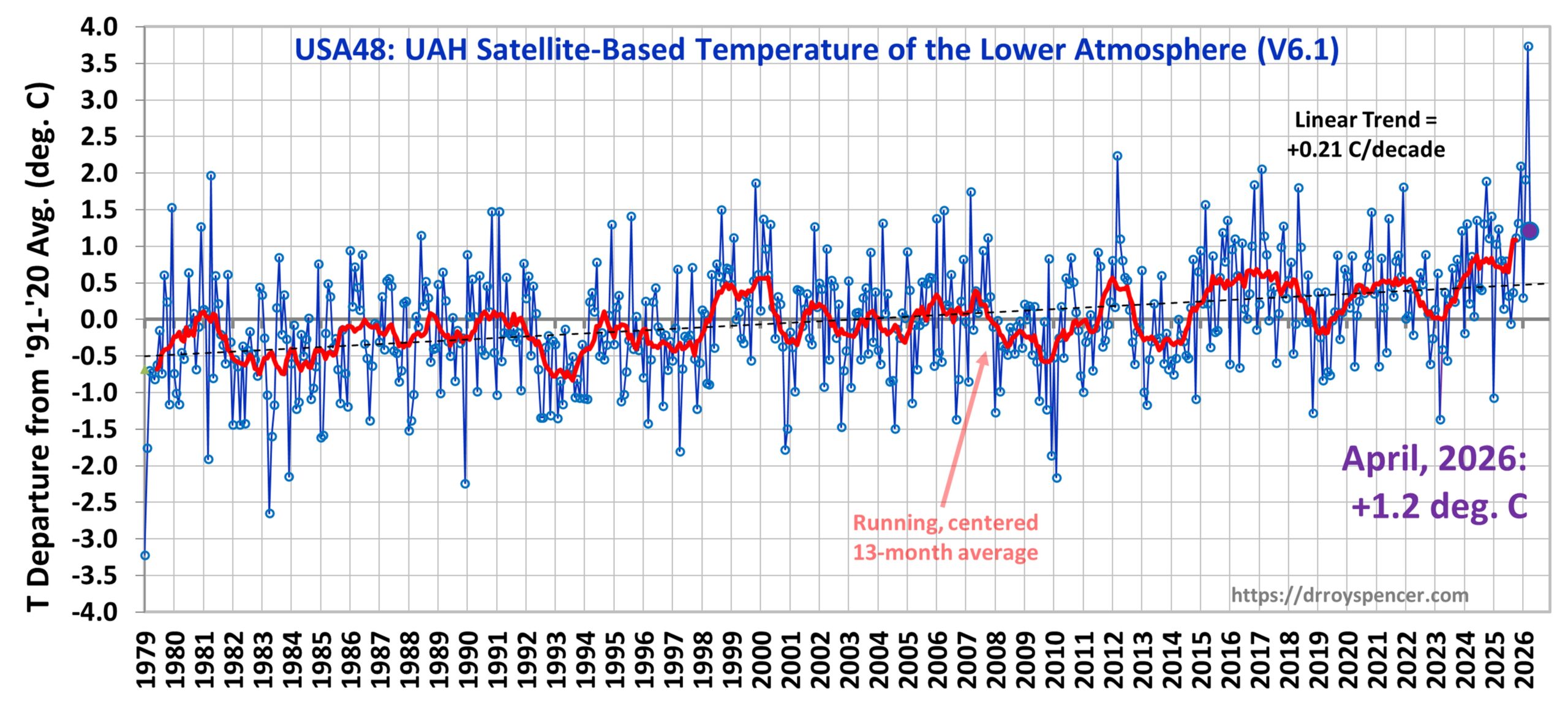
Starting this month I will include time series graphs for USA48 and Canada, in addition to the usual global plot. Note that for the previous month (March) the record warmth in USA48 (+3.74 deg. C) was in stark contrast to the coldest March in Canada in the 48-year satellite record (-3.17 deg. C).
The full UAH Global Temperature Report, along with the LT global gridpoint anomaly map for April, 2026 and a more detailed analysis by John Christy, should be available within the next several days here.
The monthly anomalies for various regions for the four deep layers we monitor from satellites will be available in the next several days at the following locations:
I’ve been spending recent months applying our novel methodology of quantifying the urban heat island (UHI) effect on surface air temperature, now using Landsat-based Impervious Surface (IS) cover fraction as a proxy for urbanization. This is an adaptation of our published research using population density (PD) as a proxy for urbanization, in which we showed that about 60% of the U.S. warming trend since the late 1800s in urban and suburban areas could be attributed to increases in population density. We used non-homogenized (raw) GHCN temperature data in that study; it remains unknown to what extent homogenization procedures implemented by NOAA, Berkeley BEST, et al. have removed this spurious warming effect.
One important aspect of the population density-based research was that the UHI effect on U.S. warming trends largely disappeared after about 1960. We used population density for that study because there are global gridpoint datasets of PD at approximately 10 km spatial resolution going back centuries. So, it was a data availability choice.
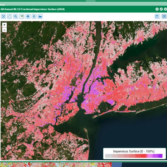
But the more physically direct proxy for urbanization in the context of the UHI effect is how much of the surface is covered by impervious surfaces (mainly roads, parking lots, buildings, etc). There are now Landsat-based datasets of IS coverage over the U.S. at high spatial resolution (~30 m) but only since 1985 when Landsat data quality was sufficient for such retrievals. This post addresses some results using those IS data. Here’s an example of IS data for the NYC area in 2024:
Fig. 1. Landsat-based impervious surface (IS) cover fraction for the New York City area based upon 2024 data. (Source: https://www.mrlc.gov/viewer/).
Specifically, I’m going through the top major Metropolitan Statistical Areas (MSAs) ranked by total population to quantify the average summertime (JJA) UHI impact on daily maximum temperature (Tmax) and minimum temperature (Tmin). I’m computing these effects separately for excessively hot days (~97th percentile) versus non-excessively hot days, which is yielding some interesting results. The analyses are based upon all available GHCN daily data during the summers of 1985 through 2025 within 40 to 100 km of the approximate centroidal location of the major metropolitan areas.
The Surprising (to me) Impact of Elevation, Nighttime Watering, and Daytime Ocean- and Lake-Breezes
Elevation
One thing I enjoy about analyzing large datasets is when I find something that surprises me… even when it shouldn’t have surprised me. The first effect was elevation. We all know that temperature decreases with height in the troposphere. This is why other UHI studies have required urban thermometer locations to be at elevations not very different from the rural locations. The “gold standard” requirement has been no more than 10 m or 30 m difference in elevation.
The problem with this standard is that it greatly restricts the number of available GHCN stations being analyzed. Since the UHI effect is often not much more different from station-specific biases due to other factors, one needs as many stations as possible to beat down the noise and extract the UHI signal. I have been using a rather loose 100 m to 250 m, but I gradually realized this was causing a bias in the results.
Why a bias, rather than just elevation difference-related noise? As I went down the list of the top U.S. metropolitan areas I realized that virtually all of them have something in common: they are at average elevations lower than the surrounding rural areas. This makes sense historically since major cities were originally developed next to major water bodies to factilitate transportation: the ocean, major rivers, and large lakes, which are all at lower elevations than their surroundings. This means that a portion of what we perceive to be the urban heat island effect is often due to differences in elevation. Sometimes there isn’t a major water body (e.g. Las Vegas), but for several practical reasons cities are seldom built in the mountains; they are instead in the low-lands.
So, I implemented a multiple regression procedure to separate out the impact of elevation from impervious surface cover in my calculations. This allows me to use all available stations, no matter their elevation, which helps to beat down the noise from other, non-UHI effects on measured air temperatures.
Nighttime Watering
I also found that most of the western U.S. cities have curious UHI effects, expecially during excessively hot days. Most of the U.S. West is characterized by summertime drought as a persistent feature of the weather there. I am now pretty sure that in many of these cases the curious results are due to nighttime watering of vegetation, which increases during excessively hot days.
Ocean and Lake Breezes
Several major cities experience significant daytime ocean breezes (e.g. Los Angeles) or lake breezes (e.g. Chicago). This acts against the urban heat island warming. As we will see, in the case of Los Angeles the cooling sea breeze almost totally dominates over any UHI warming.
Some Major Metropolitan Area Results
My methodology uses all available GHCN station pairs available on each summer day for the years 1985 through 2025. For each station pair, I compute the temperature differences (Tmax and Tmin, separately), as well as the differences in 1×1 km average impervious surface coverage centered on those station locations (I also looked at 2×2, 5×5, and 10×10 km results). This is done for all station pairs within 40 km to 100 km (city-dependent) of the approximate centroid of the MSA being considered (in the case of NYC, I chose Central Park). I then group all of these station-paired data into 7 classes of 2-station average IS coverage, which allows me to examine any nonlinearities in the UHI-vs-IS relationships. For each class, I regress the temperature differences against the IS differences to get an average dT/dIS (regression slope) value. These 7 slopes are then integrated across IS to arrive at curves of UHI temperature impact versus IS.
An important feature of the method is that I don’t have to categorize a station as “rural” or “urban”, as most other UHI studies have done. As seen in Fig. 1 (above) there is a continuum of urbanization as quantified by IS coverage from 0% (wilderness) to 100% (complete coverage by roads, parking lots, buildings, etc.)
New York City-Newark-Jersey City MSA
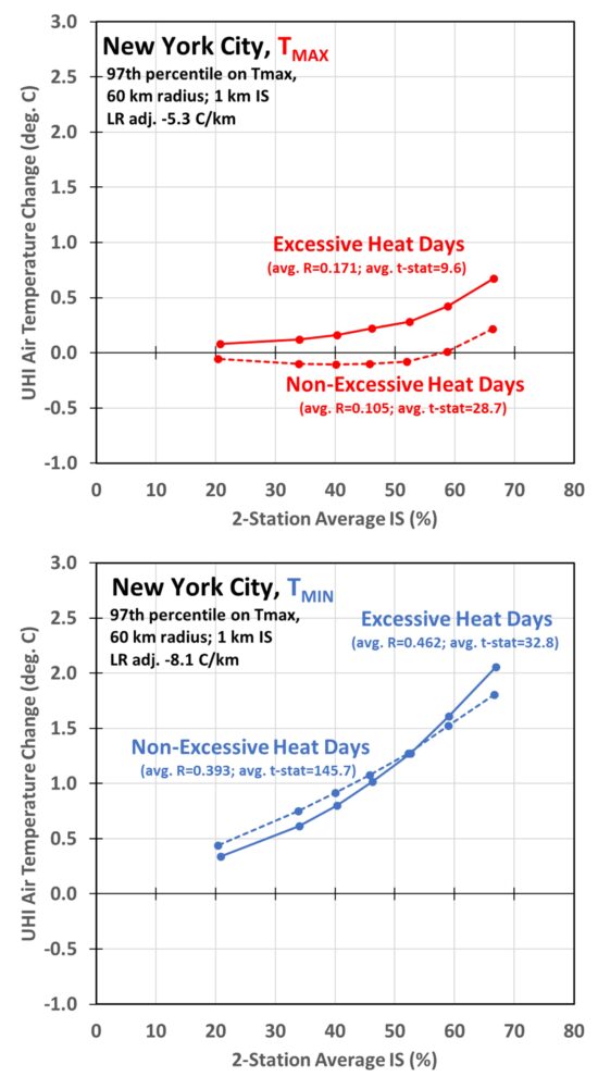
The New York-Newark-Jersey City MSA is the most populous in the U.S., with 6% of the U.S. population residing there. Fig. 2 shows the resulting average UHI effects across this MSA on Tmax and Tmin, and for excessively-hot days vs. not excessively hot days.
Fig. 2. Calculated UHI air temperature dependence on 1×1 km impervious surface coverage for the New York City-Newark-Jersey City metropolitan statistical area (MSA) based upon all GHCN station pairs within 60 km of Central Park. The regression-derived temperature lapse rate adjustments used to correct for station elevation differences are listed, as are the 7-class average correlaion coefficients and regression t-statistics. There were a total of 943,907 daily station pairs analyzed for the non-excessive heat days, and 34,469 daily station pairs for the excessive heat days.
(It is important to point out that these results should not be interpreted as necessarily representing inner-city NYC vs. surrounding rural areas. They are the average results for all available station pairs found within 60 km of Central Park, thus are for stations generally not in downtown NYC. Instead, they provide an average picture of how urbanization affects air temperatures, on average, across the entire metropolitan region.)
The first thing we see in Fig. 2 is that the UHI warming effects are much larger on Tmin than on Tmax, which many others have found.
Secondly, we see that excessively hot days have a somewhat stronger UHI warming effect at the most urbanized locations (largest IS values). But for Tmax on non-excessively hot days there is evidence of the “urban cool island” effect, which others have studied and published results on. This is a natural consequence of impervious surfaces conducting heat down into the sub-surface compared to natural land (and vegetation) surfaces, which causes a time lag in the diurnal temperature response.
Los Angeles-Long Beach-Anaheim MSA
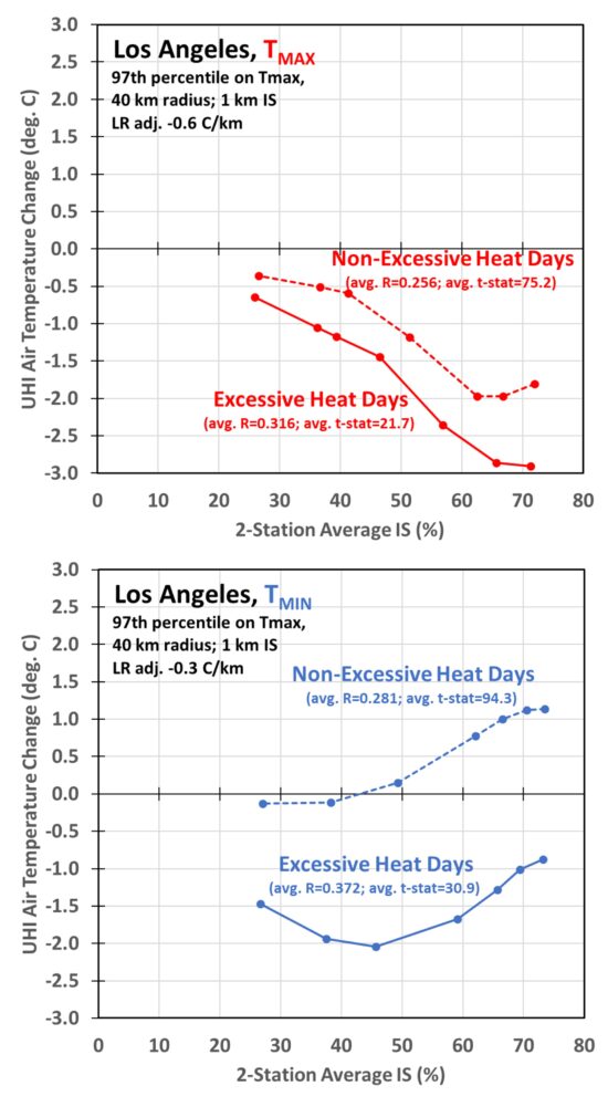
We need only go to the 2nd most populous MSA (Los Angeles) to see that the temperature changes in urban areas are not always due to warming from urbanization. This is shown in Fig. 3.
Fig. 3. As in Fig. 2, but for all GHCN station pairs within 40 km of downtown Los Angeles.
In this case we see a huge daytime cooling effect on Tmax in urban areas, which I assume is due to the persistent daytime sea breeze in the LA basin during summer. The effect is also seen to a lesser extent in Tmin for excessively hot days. I don’t know whether this is due to stronger and more persistent sea breezes on excessively hot days, or due to more nighttime watering of vegetation during those days, or some combination of both.
At this point you might be wondering, how can the hottest days have cooler urban temperatures? This is where I have to explain how I classify “excessively hot days”. Because there are so many GHCN stations within 40 km of downtown LA, there are days when some stations exceed their 97th percentile hottest temperature and other stations do not. So how do we decide which days are “excessively hot” for the metropolitan region as a whole? I calculate for each date in the summers of 1985-2025 how many stations exceed their 97th percentile threshold. I then compute the average daily temperature across those stations. For LA, it turns out at least 12 stations exceeding their 97th percentile temperature threshold are required in order for approximately 3% of the dates to be categorized as “excessively hot”, thus providing a 97th percentile threshold for the whole MSA region. I then use that 12-station minimum, applied to Tmax (not Tmin), to decide which dates are “excessively hot”.
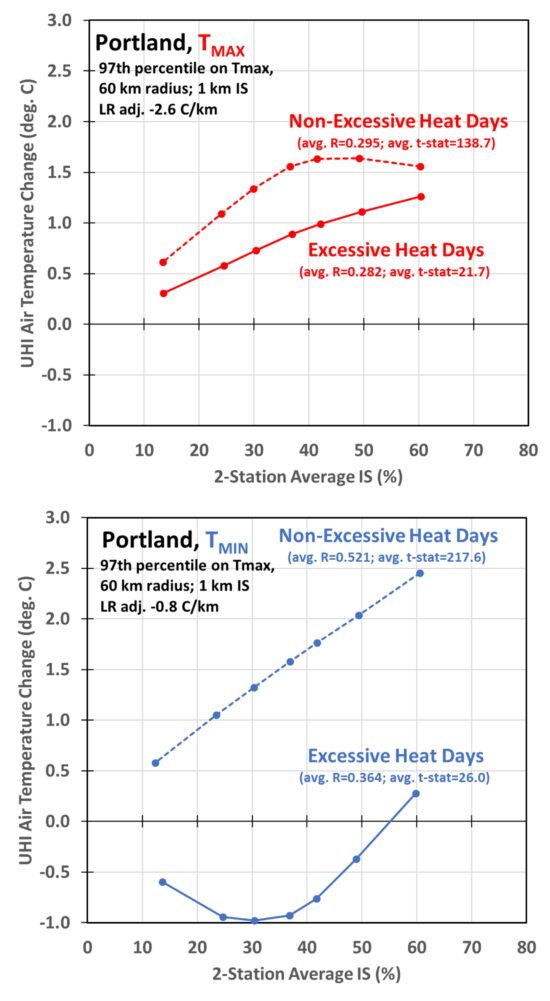
I am finding that most of the major cities in the western U.S. have reduced UHI heating (and like LA, even cooling) during daytime and nighttime on excessively hot days. In many cases I believe this is due to watering of vegetation, which for every city I have checked, Grok says that city has more water usage during the nighttime hours on excessively hot days. For example, here are the results for Portland-Vancouver-Hillsboro, the 24th most populous MSA in the U.S; note how the fairly strong UHI warming effect on Tmax and Tmin is reduced on the hottest days, especially at night when most watering occurs:
Fig. 4. As in Fig. 2, but for all station pairs within 60 km of downtown Portland, Oregon.
For the bottom curve in Fig. 4 (nighttime Portland temperatures on excessively hot dates), one might even imagine the maximum cooling effect from more watering is in the suburbs (IS less than 20-30%), but then switching to warming in the most urban areas (IS over 50%), presumably due to differences in areal coverage by vegetation being watered.
I am through about two dozen of the 50 most populous metropolitan areas I want to include results for as part of a paper we are preparing for submission to the journal Urban Climate. Since those 50 MSAs include over 50% of the U.S. population, chances are good your city or town will also be included.
The Version 6.1 global average lower tropospheric temperature (LT) anomaly for March, 2026 was +0.38 deg. C departure from the 1991-2020 mean, statistically unchanged from the February, 2026 value of +0.39 deg. C.
The Version 6.1 global area-averaged linear temperature trend (January 1979 through March 2026) remains at +0.16 deg/ C/decade (+0.22 C/decade over land, +0.13 C/decade over oceans).
The following table lists various regional Version 6.1 LT departures from the 30-year (1991-2020) average for the last 27 months (record highs are in red).
YEAR
MO
GLOBE
NHEM
SHEM
TROPIC
USA48
ARCTIC
AUST
2024
Jan
+0.80
+1.02
+0.57
+1.20
-0.19
+0.40
+1.12
2024
Feb
+0.88
+0.94
+0.81
+1.16
+1.31
+0.85
+1.16
2024
Mar
+0.88
+0.96
+0.80
+1.25
+0.22
+1.05
+1.34
2024
Apr
+0.94
+1.12
+0.76
+1.15
+0.86
+0.88
+0.54
2024
May
+0.77
+0.77
+0.78
+1.20
+0.04
+0.20
+0.52
2024
June
+0.69
+0.78
+0.60
+0.85
+1.36
+0.63
+0.91
2024
July
+0.73
+0.86
+0.61
+0.96
+0.44
+0.56
-0.07
2024
Aug
+0.75
+0.81
+0.69
+0.74
+0.40
+0.88
+1.75
2024
Sep
+0.81
+1.04
+0.58
+0.82
+1.31
+1.48
+0.98
2024
Oct
+0.75
+0.89
+0.60
+0.63
+1.89
+0.81
+1.09
2024
Nov
+0.64
+0.87
+0.40
+0.53
+1.11
+0.79
+1.00
2024
Dec
+0.61
+0.75
+0.47
+0.52
+1.41
+1.12
+1.54
2025
Jan
+0.45
+0.70
+0.21
+0.24
-1.07
+0.74
+0.48
2025
Feb
+0.50
+0.55
+0.45
+0.26
+1.03
+2.10
+0.87
2025
Mar
+0.57
+0.73
+0.41
+0.40
+1.24
+1.23
+1.20
2025
Apr
+0.61
+0.76
+0.46
+0.36
+0.81
+0.85
+1.21
2025
May
+0.50
+0.45
+0.55
+0.30
+0.15
+0.75
+0.98
2025
June
+0.48
+0.48
+0.47
+0.30
+0.80
+0.05
+0.39
2025
July
+0.36
+0.49
+0.23
+0.45
+0.32
+0.40
+0.53
2025
Aug
+0.39
+0.39
+0.39
+0.16
-0.06
+0.82
+0.11
2025
Sep
+0.53
+0.56
+0.49
+0.35
+0.38
+0.77
+0.30
2025
Oct
+0.53
+0.52
+0.55
+0.24
+1.12
+1.42
+1.67
2025
Nov
+0.43
+0.59
+0.27
+0.24
+1.32
+0.78
+0.36
2025
Dec
+0.30
+0.45
+0.15
+0.19
+2.10
+0.32
+0.37
2026
Jan
+0.35
+0.51
+0.19
+0.09
+0.30
+1.40
+0.95
2026
Feb
+0.39
+0.54
+0.23
+0.03
+1.91
-0.48
+0.73
2026
Mar
+0.38
+0.33
+0.42
+0.07
+3.74
-0.48
+1.14
YEAR
MO
GLOBE
NHEM
SHEM
TROPIC
USA48
ARCTIC
AUST
Record Warmth in the Contiguous U.S. (Lower 48)
For the Lower 48, the March 2026 temperature anomaly was easily the record warmest of all months in the 47+ year satellite record: +3.7 deg. C above average for all Marches. Second place goes to March 2012, with +2.2 deg. C above the mean, while 3rd place goes to December 2025 at +2.1 deg. C.
Interestingly, December through April are periods of large variability for the Lower 48. All 6 of the warmest months (in terms of departures from normal) since 1979 occurred in December through April. Furthermore, all 8 of the coldest months occurred in December through April.
————————-
The full UAH Global Temperature Report, along with the LT global gridpoint anomaly map for March, 2026 and a more detailed analysis by John Christy, should be available within the next several days here.
The monthly anomalies for various regions for the four deep layers we monitor from satellites will be available in the next several days at the following locations:

 Home/Blog