It is a truism that any observed change in nature will be blamed by some experts on global warming (aka “climate change”, “climate crisis”, “climate emergency”).
When the Great Lakes water levels were unusually low from approximately 2000 through 2012 or so, this was pointed to as evidence that global warming was causing the Great Lakes to dry up.
Take for example this 2012 article from National Geographic, which was accompanied by this startling photo:
The accompanying text called this the “lake bottom”, as if Lake Michigan (which averages 279 feet deep) had somehow dried up.
Then in a matter of two years, low lake levels were replaced with high lake levels. The cause (analysis here) was a combination of unusually high precipitation (contrary to global warming theory) and an unusually cold winter that caused the lakes to mostly freeze over, reducing evaporation.
Now, as of this month (June, 2019), ALL of the Great Lakes have reached record high levels.
Time To Change The Story
So, how shall global warming alarmists explain this observational defiance of their predictions?
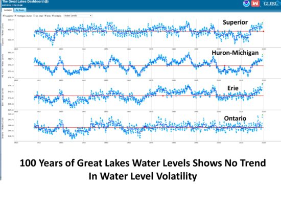
The trouble is that there is that there is no good evidence in the last 100 years that this is happening. This plot of the four major lake systems (Huron and Michigan are at the same level, connected at the Straits of Mackinac) shows no increased variability since levels have been accurately monitored (data from NOAA Great Lakes Environmental Research Laboratory):
This is just one more example of how unscientific many global warming claims have become. Both weather and climate are nonlinear dynamical systems, capable of producing changes without any ‘forcing’ from increasing CO2 or the Sun. Change is normal.
What is abnormal is blaming every change in nature we don’t like on human activities. That’s what happened in medieval times, when witches were blamed for storms, droughts, etc.
One would hope we progressed beyond that mentality.
Noctilucent (night shining) clouds are being reported farther south than ever before, with reports from southern California, New Mexico, Oklahoma, and southern Ohio.
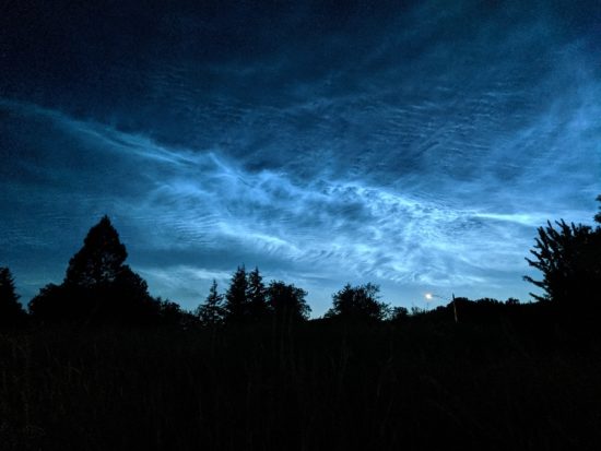
Noctilucent clouds (NLCs) over Corvallis, Oregon on June 10, 2019 (Tucker Shannon).
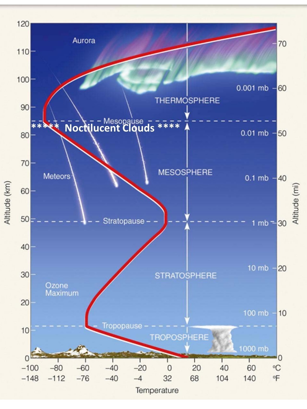
These NLCs form in the upper mesosphere at an altitude of about 85 km (around 50 miles), which is above 99.999% of the atmosphere. It is the same altitude where meteors and thunderstorm sprites occur, but somewhat below the altitude of the aurora.
Average temperature profile of the atmosphere (adapted from a presentation by Prof. Nicholas Mitchell, The University of Bath).
They are visible about 1-2 hours after sunset or before sunrise, when other clouds are in darkness but these are still illuminated by the sun due to their high altitude. It is believed that water vapor from oxidation of methane condenses on meteor dust, leading to the ice cloud formation.
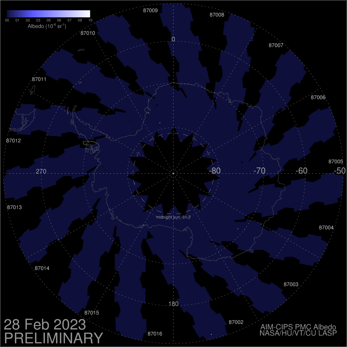
The conditions for NLC formation require extremely cold temperatures, as low as -150 deg. F. I’ve been looking for online sources of near real time satellite data which might be used to monitor them, but there isn’t much out there (more on that, below). The AIM instrument on the TIMED satellite provides daily images, but for some reason the clouds the satellite views seem to be only from the latitude of central Canada northward.
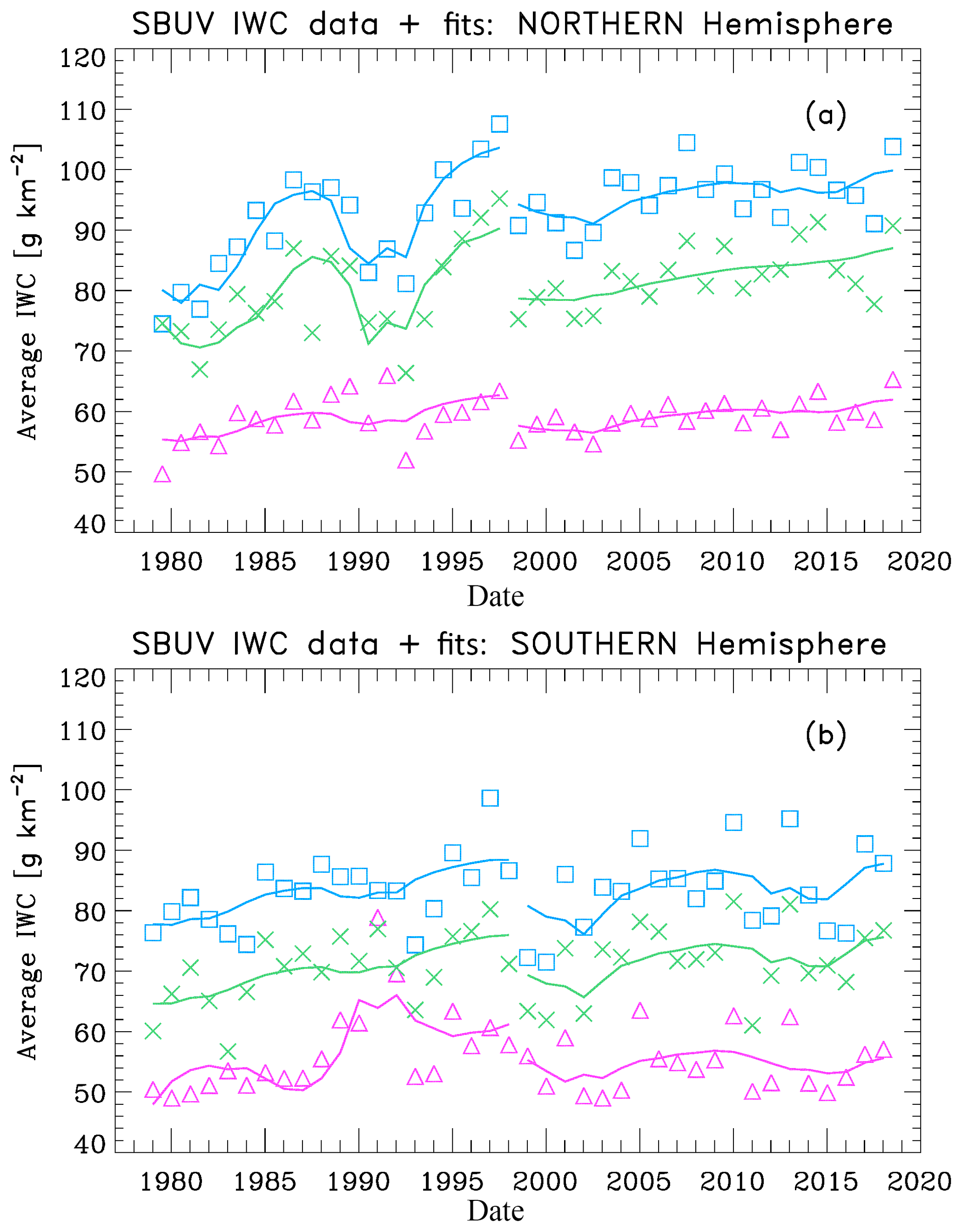
NLCs have been increasing in recent decades. They are always more prevalent during solar minimum conditions (which we are now experiencing), when there is less solar energy heating the extreme upper atmosphere. But there is also a long-term trend upward:
(a) SBUV merged seasonal average IWC (ice water content) values for three different latitude bands: 50N-64N (purple triangles), 64N-74N (green crosses) and 74N-82N (blue squares). The solid lines show multiple regression fits to the data for the periods 1979-1997 and 1998-2018. (b) SBUV merged seasonal average IWC values for 50S-64S, 64S-74S, and 74S-82S. The solid lines show fits for the periods 1979-1997 and 1998-2018. (source)
The long term increase could be the result of increasing CO2, which cools the upper atmosphere while it warms the lower atmosphere. Another possibility includes an increase in atmospheric methane, which gets oxidized into water vapor at high altitudes. Finally, some modelling suggests that climate warming should increase the Brewer-Dobson circulation, which cools the summer mesosphere (more on that, below).
Anecdotally, the most dramatic increase has been at mid-latitudes where no previous reports of NLC sightings exist. In the last couple days NLCs have been observed as far south as Joshua Tree, CA (34 deg. N) and Albuquerque, New Mexico (35 deg. N). There is no historical record of NLC sightings, anywhere, before 1880.
One of the interesting things about the mesosphere where NLCs form (and something which will mess with the heads of some here who like to argue with me) is that the summer hemisphere is colder, and the winter hemisphere warmer, in the mesosphere.
If only radiative heating by the sun (and cooling by greenhouse gases…anything that gains energy from the sun must have a way to lose that energy) were responsible for mesospheric temperatures, the opposite would be true, with the summer hemisphere being warmer, as it is in the troposphere and stratosphere.
The reason for the reversal is the Brewer-Dobson circulation, which causes upwelling (and thus adiabatic cooling) in the summer mesosphere. which That rising air forces subsidence (sinking air, and thus adiabatic warming) in the winter hemisphere.
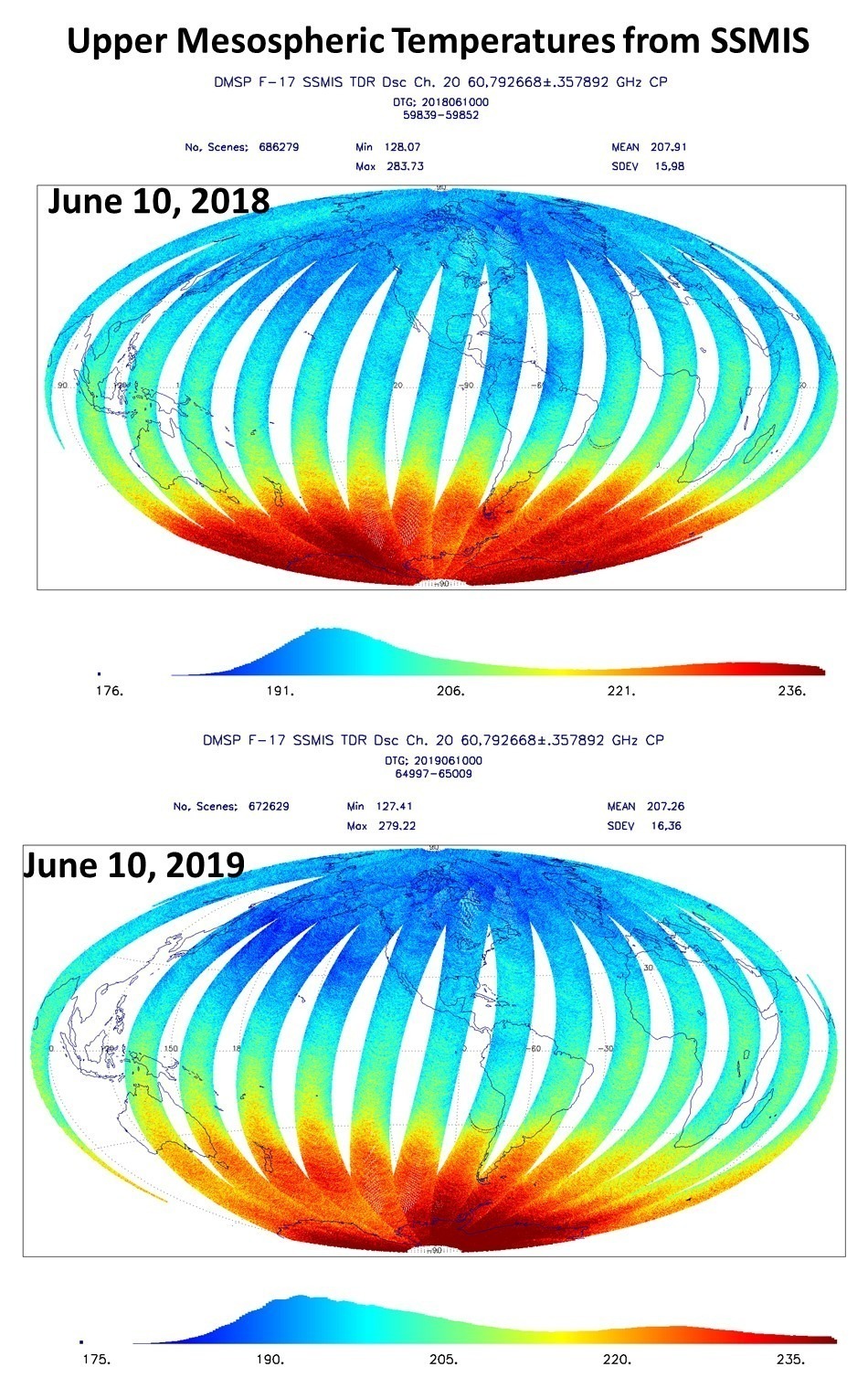
This hemispheric difference is clearly seen in upper mesospheric temperatures from channel 20 on the DMSP SSMIS instrument. These data are not widely available, and this pair of images, one year apart, was provided to me by Steve Swadley at Naval Research Laboratory – Monterey.
SSMIS imagery courtesy of Steve Swadley, NRL-Monterey.
SSMIS 60 GHz imagery of upper mesospheric temperatures one year apart shows slightly cooler temperatures in 2019 than 2018, presumably leading to more frequent noctilucent cloud sightings.
The SSMIS imagery can’t be directly related to NLC sightings because it is a vertical average for a fairly deep layer in the upper mesosphere, while NLCs form in only the very coldest layer in the upper part of that deeper layer, at the “mesopause”. But I would wager they are correlated.
I think some clever manipulation of this SSMIS channel with the one below it could provide a useful monitoring tool for NLC formation. The SSMIS instruments have been flying since before the last solar minimum, so it would be interesting to see how much colder the current solar minimum is than the last in the mesosphere. I’d love to do this myself, but considerable time would be required for data downloading, reading, analyzing, and displaying the data, and I already have a day job.
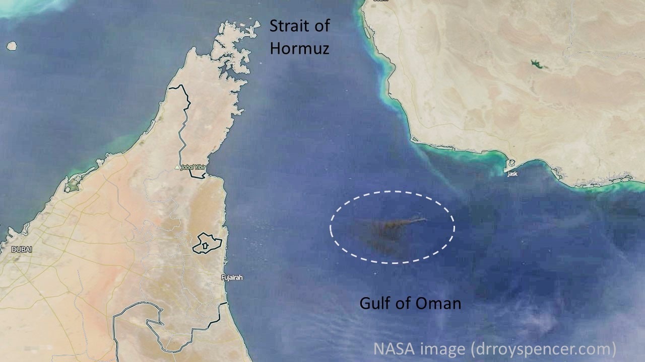
One or two oil tankers near the Strait of Hormuz were hit by torpedoes or mines this morning. I checked the NASA Worldview website to see if NASA’s MODIS imager on the Terra satellite picked it up. I had to enhance the image to bring out the dark smoke against the dark ocean background:
Over the next few weeks, mid-latitude observers might experience the best noctilucent cloud viewing of their lifetimes.
Extremely high-altitude noctilucent (night-shining) clouds viewed from Corvallis, Oregon on June 10, 2019 (Tucker Shannon, Google Pixel phone).
Observers over the northern half of the United States are reporting something they have never seen before — electric-blue noctilucent (night-shining) clouds. They are wispy in appearance, and continuously change shape. They can be seen when the sun is about 6 to 16 deg. below the horizon, so about 1 to 2 hours after sunset or before sunrise. During that time of night the sun is still shining on these clouds, but not on any normal weather-related clouds.
In the late spring every year, people at far northern latitudes have often seen these on clear or partly-cloudy evenings. But solar-minimum conditions, with few if any sunspots, are causing cooling in the extreme upper atmosphere around 80 km (~50 miles) high where the lowest atmospheric temperatures are recorded, approaching -150 deg. F (-100 deg. C). That altitude is above 99.999% of the air in the atmosphere.
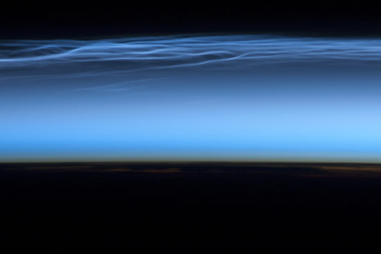
Noctilucent clouds observed from the International Space Station on June 13, 2012 (NASA).
Adding to the spectacular electric blue displays is increasing atmospheric methane, which gets converted to water vapor at these altitudes, and increasing atmospheric carbon dioxide, which causes enhanced cooling of the upper atmosphere. The result is that the conditions necessary for NLC formation are extending farther south than ever before.
The wispy and undulating appearance of the clouds is due to upward-propagating gravity (air density) waves that cause temperatures to rise and fall, and the clouds form in the colder portions of those waves. Ice grows on meteor dust particles, creating a (nearly) outer space version of cirrus clouds. Time lapse photography has been used to show how the clouds change shape as the gravity waves well up through the extremely cold upper mesosphere:
If you miss seeing them in the next several weeks, take heart — solar minimum conditions should persist until the next NLC season arrives, making the summer of 2020 a good viewing opportunity, too.
You can see recent NLC photos from around the Northern Hemisphere, updated daily, here.
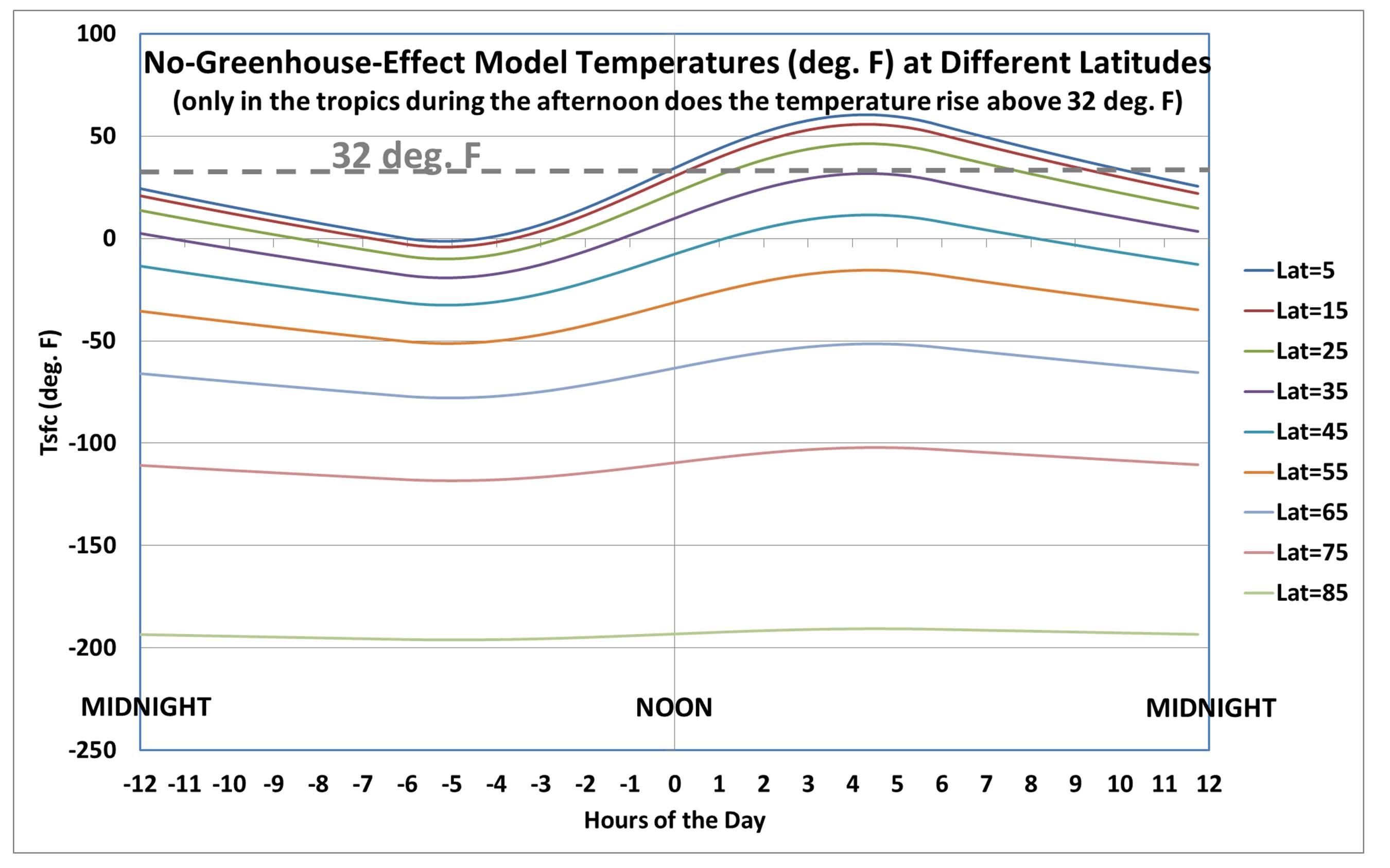
Abstract:A simple time-dependent model of Earth surface temperatures over the 24 hr day/night cycle at different latitudes is presented. The model reaches energy equilibrium after 1.5 months no matter what temperature it is initialized at. It is shown that even with 1,370 W/m2 of solar flux (reduced by an assumed albedo of 0.3), temperatures at all latitudes remain very cold, even in the afternoon and in the deep tropics. Variation of the model input parameters over reasonable ranges do not change this fact. This demonstrates the importance of the atmospheric “greenhouse” effect, which increases surface temperatures well above what can be achieved with only solar heating and surface infrared loss to outer space.
As a follow-up to yesterday’s post regarding why climate scientists use ~340 W/m2 as the global average solar flux available to the climate system, here I present a model which includes how the incident solar flux (starting with the 1,370 W/m2 solar constant) varies across the Earth as a function of latitude and every 15 minutes throughout the diurnal (day/night) cycle.
I am providing this model to avoid any objections regarding how much solar energy is input into the climate system on average, how that averaging should be done (or whether it is even physically meaningful), whether the nighttime lack of any solar flux should be excluded from the averaging, whether certain assumptions constitute a “flat-Earth” mentality, etc. Instead, the model uses the actual variations of the incident solar radiation on the (assumed spherical) Earth as a function of latitude and time of day. For simplicity, equinox conditions are assumed and so there is no seasonal cycle.
This is not meant to be a realistic model of regional climate; instead, it goes beyond the global averages in the Kiehl-Trenberth energy budget diagram and shows how unrealistically cold temperatures are when you assume there is no greenhouse effect — even in the deep tropics during the afternoon. The model “evolves” the final temperatures, from any starting temperature you specify, based upon a simple energy budget equation (energy conservation) combined with an assumed surface heat capacity. Imbalances between absorbed solar energy and emitted IR energy cause a temperature change which eventually stops (in a long-term average sense) when the daily rate of emitted IR energy equals the daily absorbed solar energy.
The time-dependent model has adjustable inputs: the solar constant (1,370 W/m2); an albedo (for simplicity assumed 0.3 everywhere); the depth of the surface layer responding to solar heating (using the heat capacity of water, but soil heat capacity is similar); and, the assumed broadband infrared emissivity of the surface controlling how fast energy is lost to space as the surface warms. I set the time step to 15 minutes to resolve the diurnal cycle. The Excel model is here, and you are free to change the input parameters and see the results.
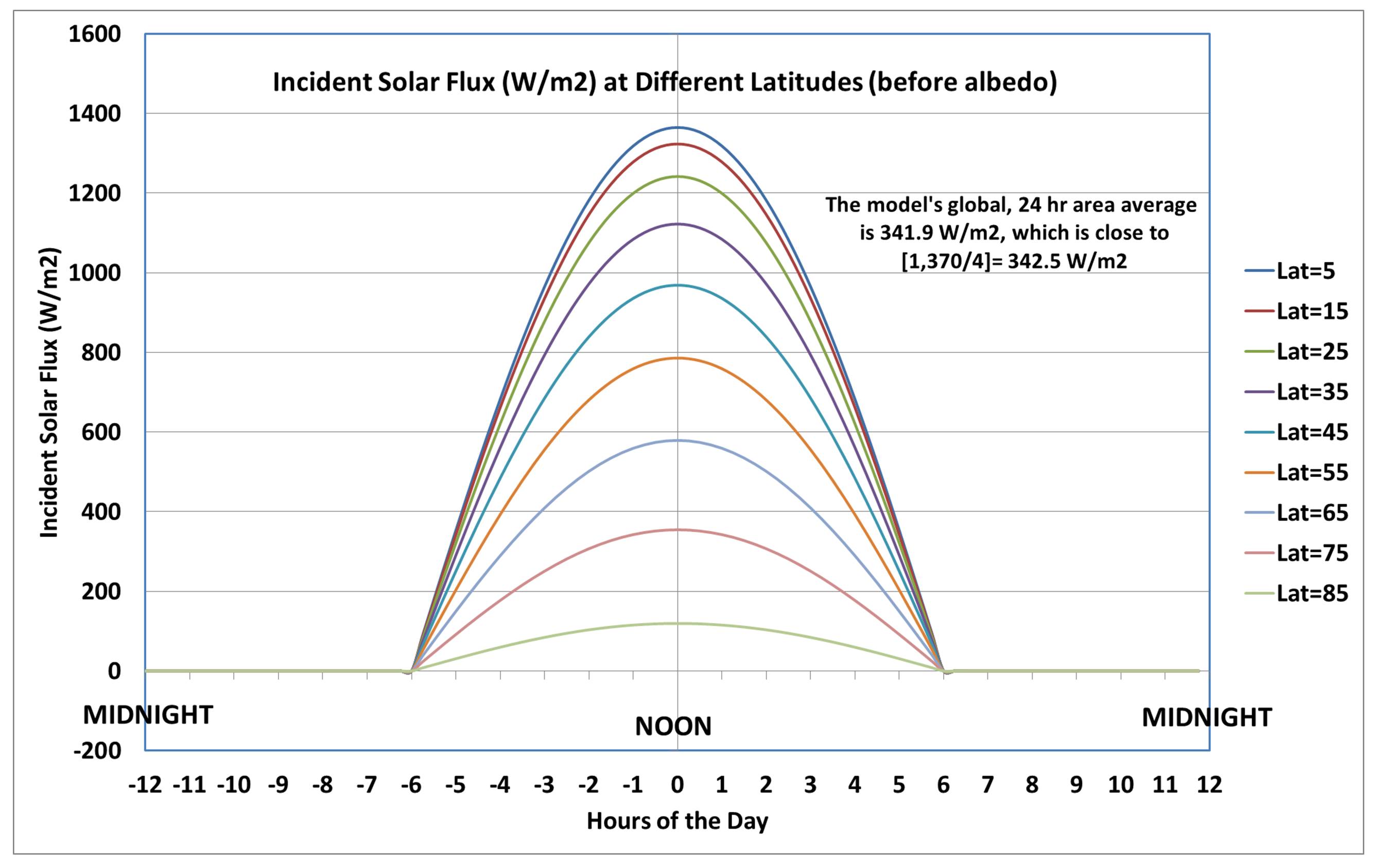
Here’s how the incident solar flux changes with time-of-day and latitude. This should not be controversial, since it is just based upon geometry. Even though I only do model calculations at latitudes of 5, 15, 25, 35, 45, 55, 65, 75, and 85 deg. (north and south), the global, 24-hr average incident solar flux is very close to simply 1,370 divided by 4, which is the ratio of the surface areas of a circle and a sphere having the same radius:
If I had done calculations for every 1 deg. of latitude, the model result would have been exceedingly close to 1,370/4.
If I assume the surface layer responding to heating is 0.1 m deep, a global albedo of 0.3, and a broadband IR emissivity of 0.98, and run the model for 46 days, the model reaches very nearly a steady-state energy equilibrium no matter what temperature I initialize it at (say, 100K or 300 K):
Note that even in the deep tropics, the average temperature is only 29 deg. F. At 45 deg. latitude, the temperature averages -11 deg. F. The diurnal temperature variations are very large, partly because the greenhouse effect in nature helps retain surface energy at night, keeping temperatures from falling too fast like it does in the model.
There is no realistic way to remove the very cold bias of the model without including an atmospheric greenhouse effect. If you object that convection has been ignored, that is a surface cooling (not warming) process, so including convection will only make matters worse. The lack of model heat transport out of the tropics, similarly, would only make the model tropical temperatures colder, not warmer, if it was included. The supposed warming caused by atmospheric pressure that some believe is an alternative theory to the GHE would cause (as Willis Eschenbach has pointed out) surface temperatures to rise, making the surface lose more energy to space than it gains from the sun, and there would no longer be energy balance, violating the 1st Law of Thermodynamics. The temperature would simply go back down again to achieve energy balance (we wouldn’t want to violate the 1st Law).
I hope this will help convince some who are still open-minded on this subject that even intense tropical sunshine cannot explain real-world tropical temperatures. The atmospheric greenhouse effect must also be included. The temperature (of anything) is not determined by the rate of energy input (say, the intensity of sunlight, or how fast your car engine burns gas); it is the result of a balance between energy gain and energy loss. The greenhouse effect reduces the rate of energy loss at the surface, thus causing higher temperatures then if it did not exist.
Willis Eschenbach and I have been defending ourselves on Facebook against Joe Postma’s claims we have “flat Earth” beliefs about the radiative energy budget of the Earth. The guy is obviously passionate, as our discussion ended with expletive-laced insults hurled my way (I suspect Willis decided the discussion wasn’t worth the effort, and withdrew before the fireworks began).
Joe advertises himself as an astrophysicist who works at the University of Calgary. I don’t know his level of education, but his claims have considerable influence on others, which is why I am addressing them here. He has numerous writings and Youtube videos on the subject of Earth’s energy budget and greenhouse effect, and the supposed errors the climate research community has made. I get emails and comments on my blog from others who invoke his claims, and so he is difficult to ignore.
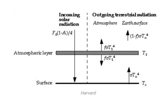
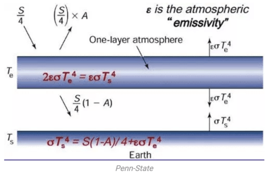
Here I want to address just one of his claims (repeated by others, and the basis of his accusation I am a flat-Earther), recently described here, regarding the value of solar flux at the top of the atmosphere that is found in many simplified diagrams of the Earth’s energy budget. I will use the same two graphics used in that article, one from Harvard and one from Penn State:
Joe’s claim (as far as I can tell) is that that the solar flux value (often quoted to be around 342 W/m2) is unrealistic because it is for a flat Earth. But as an astrophysicist, he should recognize the division by 4 (“Fs(1-A)/4” and “S/4”) in the upper-left portion of both figures, which takes the solar constant at the distance of the Earth from the sun (about 1,370 W/m2) and spreads it over the spherical shape of the Earth.Thus, the 342 W/m2 value represents a spherical (not flat) Earth.
Just because someone then draws a diagram using a flat surface representing the Earth doesn’t mean the calculation is for a “flat Earth”.
Next in that article, Joe’s (mistaken) value for the solar constant is then used to compute the resulting Earth-Sun distance implied by us silly climate scientists who believe the solar constant is 342.5 W/m2 (rather than the true value of 1,370 W/m2). He gets twice the true, known value of the Earth-Sun distance, simply because he used a solar flux that was off by a factor of 4.
Now, I find it hard to believe an actual astrophysicist could make such an elementary error. I can ignore Joe’s profane personal insults, but he ends up influencing many people, and then I have to deal with their questions individually. Sometimes it’s better if I can just point them to a blog post, which is why I wrote this.
UPDATE: (June 6, 2019): Joe Postma has posted a YouTube video rebutting my article. If you listen to him from 2:30 to 2:45, Joe refuses to accept that the S=1,370 W/m2 “solar constant” energy that is intercepted by the cross-sectional area of the Earth must then get spread out, over time, over the whole (top-of-atmosphere) surface area of Earth. [This why S gets divided by 4 in global average energy budget diagrams, it’s the difference between the area of a circle and the area of a sphere with the same radius.] I am at a loss for words how he can refuse to accept something that is so obviously true — it’s simple geometry. I stand by everything I have written here.
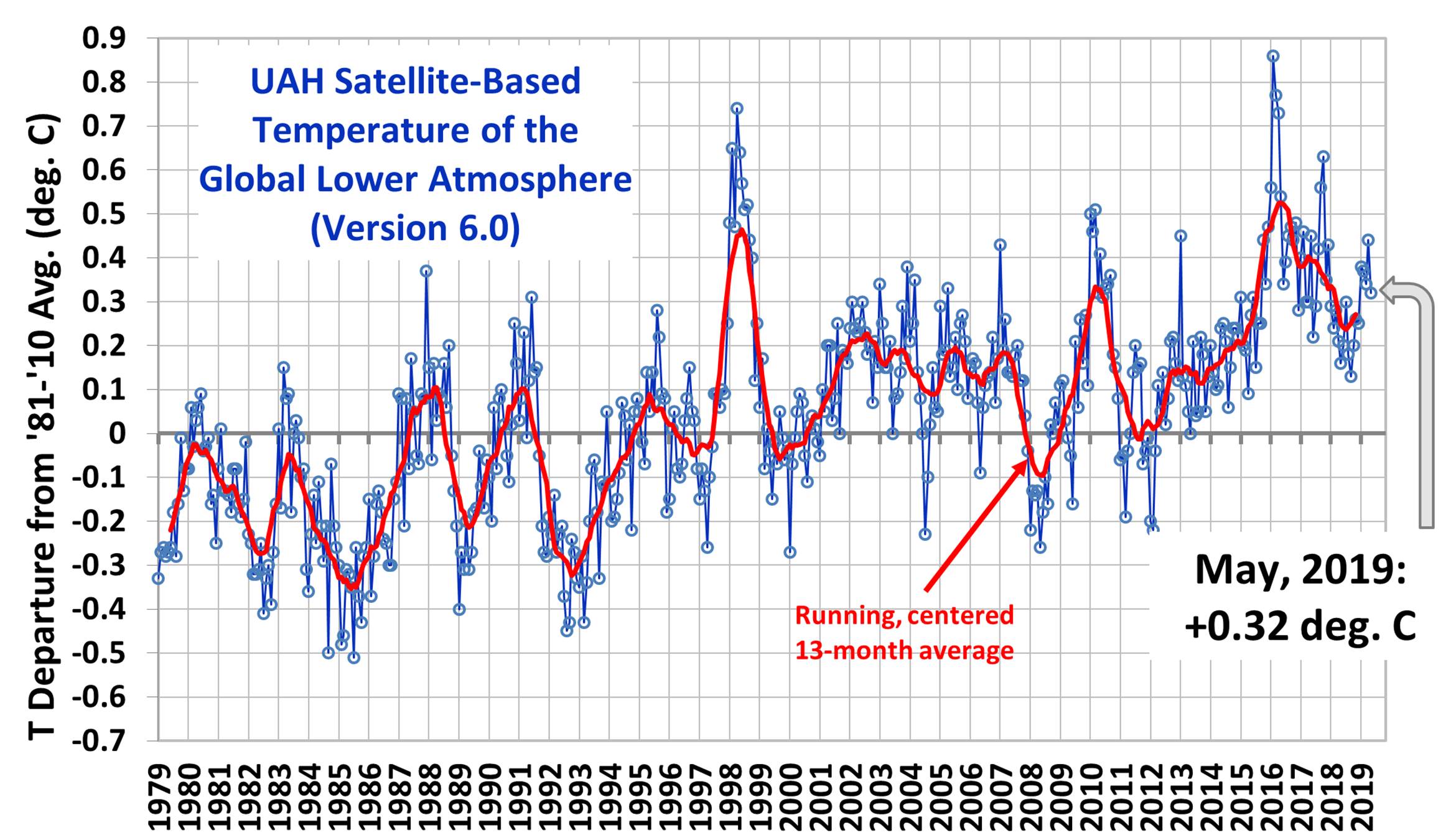
The Version 6.0 global average lower tropospheric temperature (LT) anomaly for May, 2019 was +0.32 deg. C, down from the April, 2019 value of +0.44 deg. C:
Various regional LT departures from the 30-year (1981-2010) average for the last 17 months are:

 Home/Blog


