The increasing global ocean heat content (OHC) is often pointed to as the most quantitative way to monitor long-term changes in the global energy balance, which is believed to have been altered by anthropogenic greenhouse gas emissions. The challenge is that long-term temperature changes in the ocean below the top hundred meters or so become exceedingly small and difficult to measure. The newer network of Argo floats since the early 2000s has improved global coverage dramatically.
A new Cheng et al. (2020) paper describing record warm ocean temperatures in 2019 has been discussed by Willis Eschenbach who correctly reminds us that such “record setting” changes in the 0-2000 m ocean heat content (reported in Zettajoules, which is 10^^21 Joules) amount to exceedingly small temperature changes. I calculate from their data that 2019 was only 0.004 0.009 deg. C warmer than 2018.
Over the years I have frequently pointed out that the global energy imbalance (less than 1 W/m2) corresponding to such small rates of warming is much smaller than the accuracy with which we know the natural energy flows (1 part in 300 or so), which means Mother Nature could be responsible for the warming and we wouldn’t even know it.
The Cheng (2017) dataset of 0-2000m ocean heat content changes extends the OHC record back to 1940 (with little global coverage) and now up through 2019. The methodology of that dataset uses optimum interpolation techniques to intelligently extend the geographic coverage of limited data. I’m not going to critique that methodology here, and I agree with those who argue creating data where it does not exist is not the same as having real data. Instead I want to answer the question:
If we take the 1940-2019 global OHC data (as well as observed sea surface temperature data) at face value, and assume all of the warming trend was human-caused, what does it imply regarding equilibrium climate sensitivity (ECS)?
Let’s assume ALL of the warming of the deep oceans since 1940 has been human-caused, and that the Cheng dataset accurately captures that. Furthermore, let’s assume that the HadSST sea surface temperature dataset covering the same period of time is also accurate, and that the RCP radiative forcing scenario used by the CMIP5 climate models also represents reality.
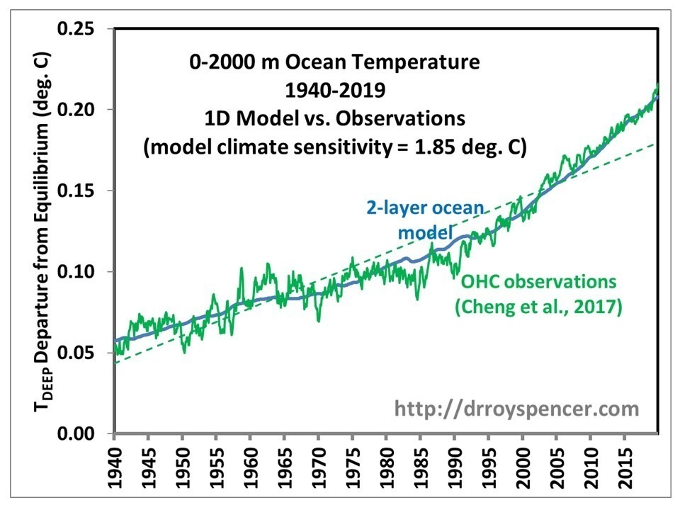
I updated my 1D model of ocean temperature with the Cheng data so that I could match its warming trend over the 80-year period 1940-2019. That model also includes El Nino and La Nina (ENSO) variability to capture year-to-year temperature changes. The resulting fit I get with an assumed equilibrium climate sensitivity of 1.85 deg. C is shown in the following figure.
Fig. 1. Deep-ocean temperature variations 1940-2019 explained with a 2-layer energy budget model forced with RCP6 radiative forcing scenario and a model climate sensitivity of 1.85 deg. C. The model also matches the 1940-2019 and 1979-2019 observed sea surface temperature trends to about 0.01 C/decade. If ENSO effects are not included in the model, the ECS is reduced to 1.7 deg. C.
Thus, based upon basic energy budget considerations in a 2-layer ocean model, we can explain the IPCC-sanctioned global temperature datasets with a climate sensitivity of only 1.85 deg. C. And even that assumes that ALL of the warming is due to humans which, as I mentioned before, is not known since the global energy imbalance involved is much smaller than the accuracy with which we know natural energy flows.
If I turn off the ENSO forcing I have in the model, then after readjusting the model free parameters to once again match the observed temperature trends, I get about 1.7 deg. C climate ECS. In that case, there are only 3 model adjustable parameters (ECS, the ocean top layer thickness [18 m], and the assumed rate or energy exchange between the top layer and the rest of the 0-2000m layer, [2.1 W/m2 per deg C difference in layer temperatures away from energy equilibrium]). Otherwise, there are 7 model adjustable parameters in the model with ENSO effects turned on.
For those who claim my model is akin to John von Neumann’s famous claim that with 5 variables he can fit an elephant and make its trunk wiggle, I should point out that none of the model’s adjustable parameters (mostly scaling factors) vary in time. They apply equally to each monthly time step from 1765 through 2019. The long-term behavior of the model in terms of trends is mainly governed by (1) the assumed radiative forcing history (RCP6), (2) the assumed rate of heat storage (or extraction) in the deep ocean as the surface warms (or cools), and (3) the assumed climate sensitivity, all within an energy budget model with physical units.
My conclusion is that the observed trends in both surface and deep-layer temperature in the global oceans correspond to low climate sensitivity, only about 50% of what IPCC climate models produce. This is the same conclusion as Lewis & Curry made using similar energy budget considerations, but applied to two different averaging periods about 100 years apart rather than (as I have done) in a time-dependent forcing-feedback model.
In 2017, Christy & McNider published a study where they estimated and removed the volcanic effects from our UAH lower tropospheric (LT) temperature record, finding that 38% of the post-1979 warming trend was due to volcanic cooling early in the record.
Yesterday in my blog post I showed results from a 1D 2-layer forcing-feedback ocean model of global-average SSTs and deep-ocean temperature variations up through 2019. The model is forced with (1) the RCP6 radiative forcings scenario (mostly increasing anthropogenic greenhouse gases and aerosols and volcanoes) and (2) the observed history of El Nino and La Nina activity as expressed in the Multivariate ENSO Index (MEI) dataset. The model was optimized with adjustable parameters, with two of the requirements being model agreement with the HadSST global temperature trend during 1979-2019, and with deep-ocean (0-2000m) warming since 1990.
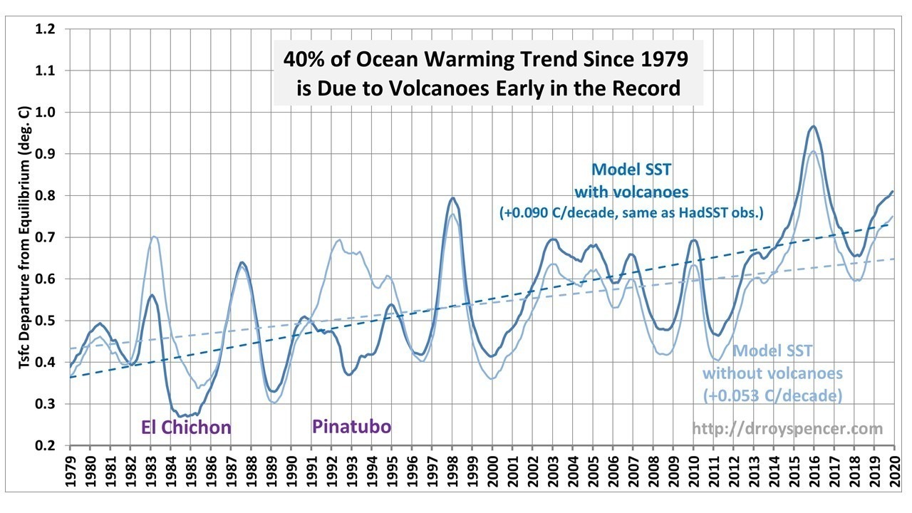
Since the period since 1979 is of such interest, I re-ran the model with the RCP6 volcanic aerosol forcing estimates removed. The results are shown in Fig. 1.
Fig. 1. 1D model simulation of global (60N-60S) average sea surface temperature departures from assumed energy equilibrium (in 1765), with and without the RCP6 volcanic radiative forcings included.
The results show that 41% of the ocean warming in the model was simply due to the two major volcanoes early in the record. This is in good agreement with the 38% estimate from the Christy & McNider study.
It is interesting to see the “true” warming effects of the 1982-83 and 1991-1993 El Nino episodes, which were masked by the eruptions. The peak model temperatures in those events were only 0.1 C below the record-setting 1997-98 El Nino, and 0.2 C below the 2015-16 El Nino.
This is not a new issue, of course, as Christy & McNider also published a similar analysis in Nature in 1994.
These volcanic effects on the post-1979 warming trend should always be kept in mind when discussing the post-1979 temperature trends.
NOTE: In a previous version of this post I suggested that the Christy & McNider (1994) paper had been scrubbed from Google. It turns out that Google could not find it if the authors’ middle initials were included(but DuckDuckGo had no problem finding it).
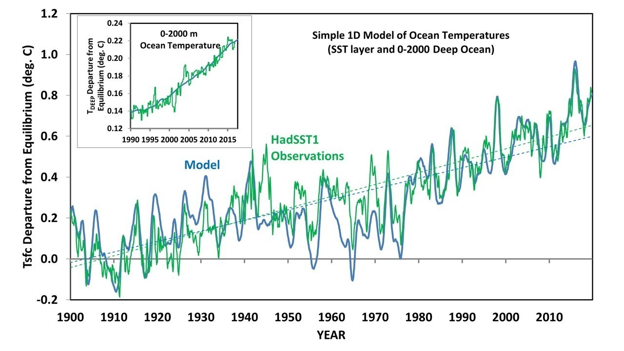
The continuing global-average warmth over the last year has caused a few people to ask for my opinion regarding potential explanations. So, I updated the 1D energy budget model I described a couple years ago here with the most recent Multivariate ENSO Index (MEIv2) data. The model is initialized in the year 1765, has two ocean layers, and is forced with the RCP6 radiative forcing scenario and the history of El Nino and La Nina activity since the late 1800s.
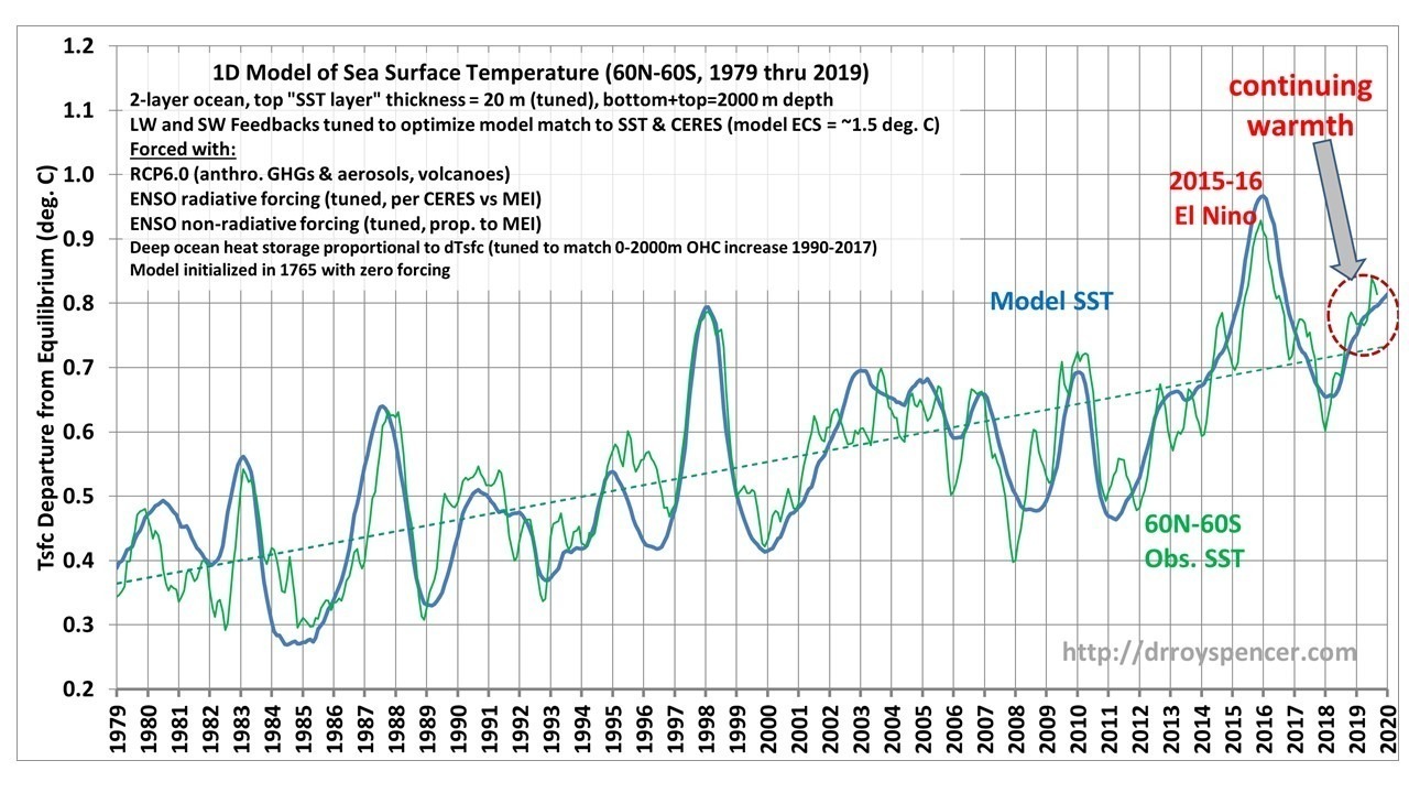
The result shows that the global-average (60N-60S) ocean sea surface temperature (SST) data in recent months are well explained as a reflection of continuing weak El Nino conditions, on top of a long-term warming trend.
Fig. 1. 1D model of global ocean temperatures compared to observations. The model is forced with the RCP6 radiative forcing scenario (increasing CO2, volcanoes, anthropogenic aerosols, etc.) and the observed history of El Nino and La Nina since the late 1800s. The observations are monthly running 3-month averages and are offset with a single bias to match the model temperatures, which are departures from assumed energy equilibrium in 1765.
The model is described in more detail below, but here I have optimized the feedbacks and rate of deep ocean heat storage to match the 41-year warming trend during 1979-2019 and increase in 0-2000m ocean heat content during 1990-2017.
While the existence of a warming trend in the current model is due to increasing CO2 (I use the RCP6 radiative forcing scenario), I agree that natural climate variability is also a possibility, or (in my opinion) some combination of the two. The rate of deep-ocean heat storage since 1990 (see Fig. 3, below) represents only 1 part in 330 of global energy flows in and out of the climate system, and no one knows whether there exists a natural energy balance to that level of accuracy. The IPCC simply *assumes* it exists, and then concludes long-term warming must be due to increasing CO2. The year-to-year fluctuations are mostly the result of the El Nino/La Nina activity as reflected in the MEI index data, plus the 1982 (El Chichon) and 1991 (Pinatubo) major volcanic eruptions.
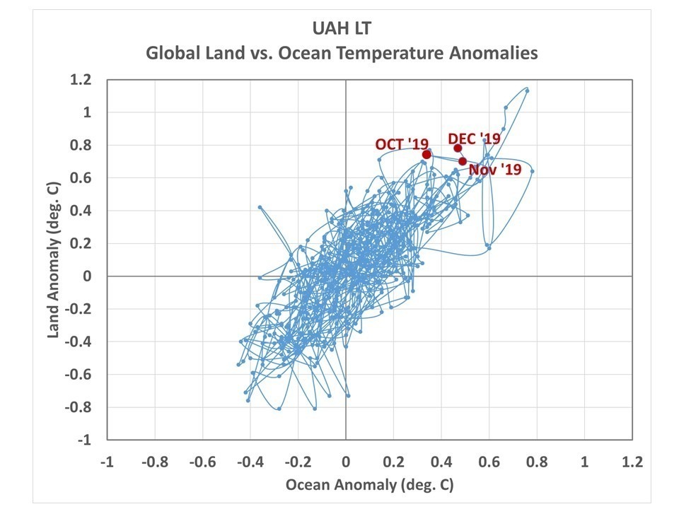
When I showed this to John Christy, he asked whether the land temperatures have been unusually warm compared to the ocean temperatures (the model only explains ocean temperatures). The following plot shows that for our UAH lower tropospheric (LT) temperature product, the last three months of 2019 are in pretty good agreement with the rest of the post-1979 record, with land typically warming (and cooling) more than the ocean, as would be expected for the difference in heat capacities, and recent months not falling outside that general envelope. The same is true of the surface data (not shown) which I have only through October 2019.
Fig. 2. UAH lower tropospheric temperature departures from the 1981-2010 average for land versus ocean, 1979 through 2019.
The model performance since 1900 is shown next, along with the fit of the model deep-ocean temperatures to observations since 1990. Note that the warming leading up to the 1940s is captured, which in the model is due to stronger El Nino activity during that time.
Fig. 3. As in Fig. 1, but for the period 1900-2019. The inset show the model versus observations for the increase in 0-2000 m ocean temperatures since 1990.
The model equilibrium climate sensitivity which provides the best match to the observational data is only 1.54 deg. C, using HadSST1 data. If I use HadSST3 data, the ECS increases to 1.7 deg. C, but the model temperature trends 1880-2019 and 1979-2019 can no longer be made to closely approximate the observations. This suggests that the HadSST1 dataset might be a more accurate record than HadSST3 for multi-decadal temperature variability, although I’m sure other explanations could be envisioned (e.g. errors in the RCP6 radiative forcing, especially from aerosol pollution).
A Brief Review of the 1D Model
The model is not just a simple statistical fit of observed temperatures to RCP6 and El Nino/La Nina data. Instead, it uses the energy budget equation to compute the monthly change in temperature of ocean near-surface layer due to changes in radiative forcing, radiative feedback, and deep-ocean heat storage. As such, each model time step influences the next model time step, which means the model adjustable parameters cannot be optimized by simple statistical regression techniques. Instead, changes are manually made to the adjustable model parameters, the model is run, and then compared to a variety of observations (SST, deep ocean temperatures, and how CERES radiative fluxes vary with the MEI index). Many combinations of model adjustable parameters will give a reasonably good fit to the data, but only within certain bounds.
There are a total of seven adjustable parameters in the model, and five time-dependent datasets whose behavior is explained with various levels of success by the model (HadSST, NODC 0-2000m deep ocean temperature [1990-2017], and the lag-regression coefficients of MEI versus CERES satellite SW, LW, and Net radiative fluxes [March 2000 through April 2019]).
The model is initialized in 1765 (when the RCP6 radiative forcing dataset begins) which is also when the climate system is (for simplicity) assumed to be in energy balance. Given the existence of the Little Ice Age, I realize this is a dubious assumption.
The energy budget model computes the monthly change in temperature (dT/dt) due to the RCP6 radiative forcing scenario (which starts in 1765, W/m2) and the observed history of El Nino and La Nina activity (starting in 1880 from the extended MEI index, intercalibrated with and updated to the present with the newer MEIv2 dataset (W/m2 per MEI value, with a constant of proportionality that is consistent with CERES satellite observations since 2000). As I have discussed before, from CERES satellite radiative budget data we know that El Nino is preceded by energy accumulation in the climate system, mainly increasing solar input from reduced cloudiness, while La Nina experiences the opposite. I use the average of the MEI value in several months after current model time dT/dt computation, which seems to provide good time phasing of the model with the observations.
Also, an energy conserving non-radiative forcing term is included, proportional to MEI at zero time lag, which represents the change in upwelling during El Nino and La Nina, with (for example) top layer warming and deep ocean cooling during El Nino.
A top ocean layer assumed to represent SST is adjusted to maximize agreement with observations for short-term variability, and as the ocean warms above the assumed energy equilibrium value, heat is pumped into the deep ocean (2,000 m depth) at a rate that is adjusted to match recent warming of the deep ocean.
Empirically-adjusted longwave IR and shortwave solar feedback parameters represent how much extra energy is lost to outer space as the system warms. These are adjusted to provide reasonable agreement with CERES-vs.-MEI data during 2000-2019, which are a combination of both forcing and feedback related to El Nino and La Nina.
Generally speaking, changing any one of the adjustable parameters requires changes in one or more of the other parameters in order for the model to remain reasonably close to the variety of observations. There is no one “best” set of parameter choices which gives optimum agreement to the observations. All reasonable choices produce equilibrium climate sensitivities in the range of 1.4 to 1.7 deg. C.
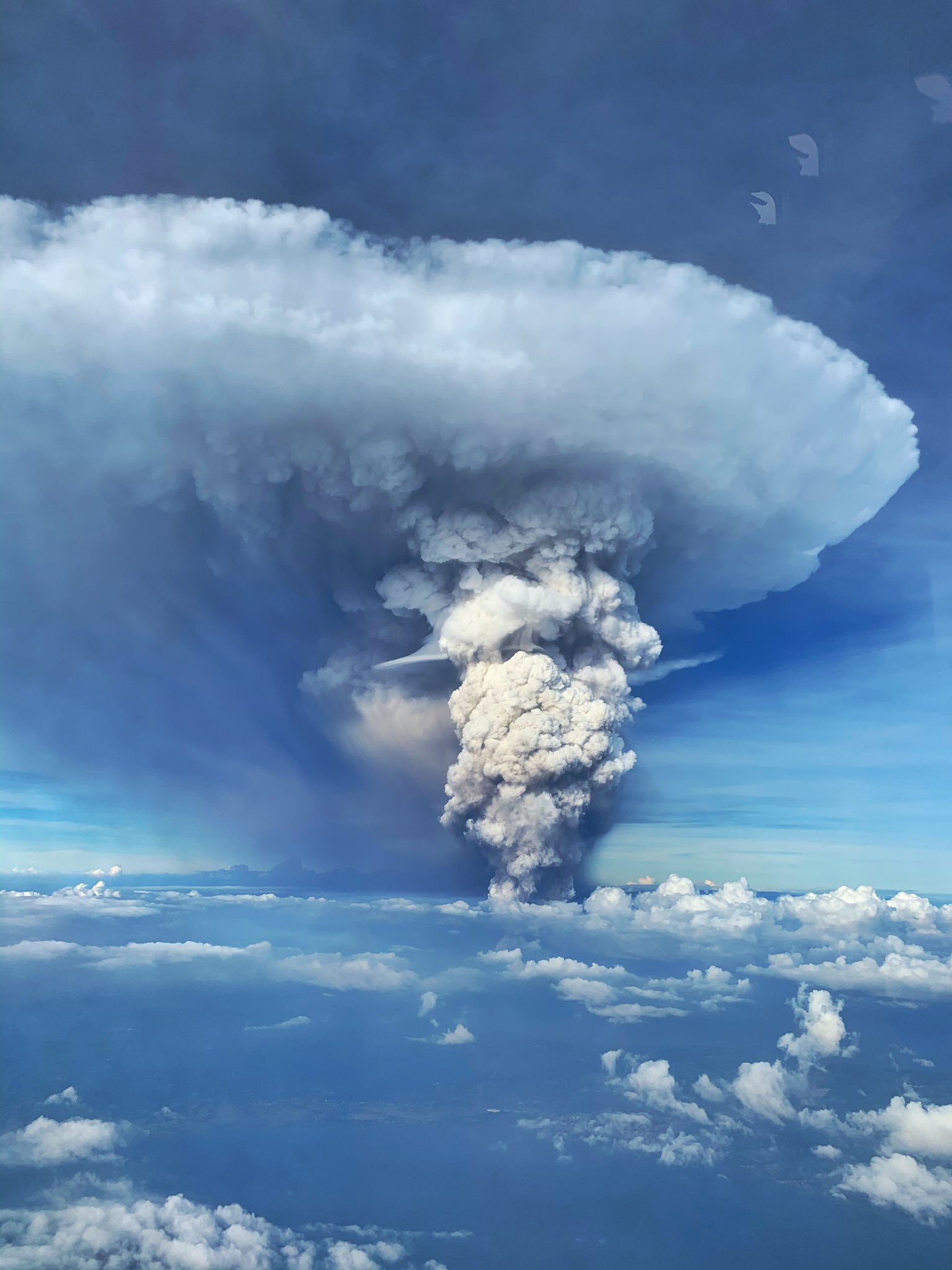
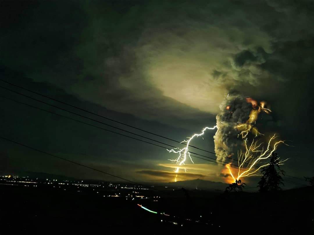
The sudden eruption of Taal volcano south of Manila, Philippines began about 0630 UTC today, and the Himawari-8 satellite infrared imagery suggests that the plume might have penetrated the stratosphere, which is necessary for the volcano to have any measurable effect on global temperatures. The following link will take you to the recent satellite loop.
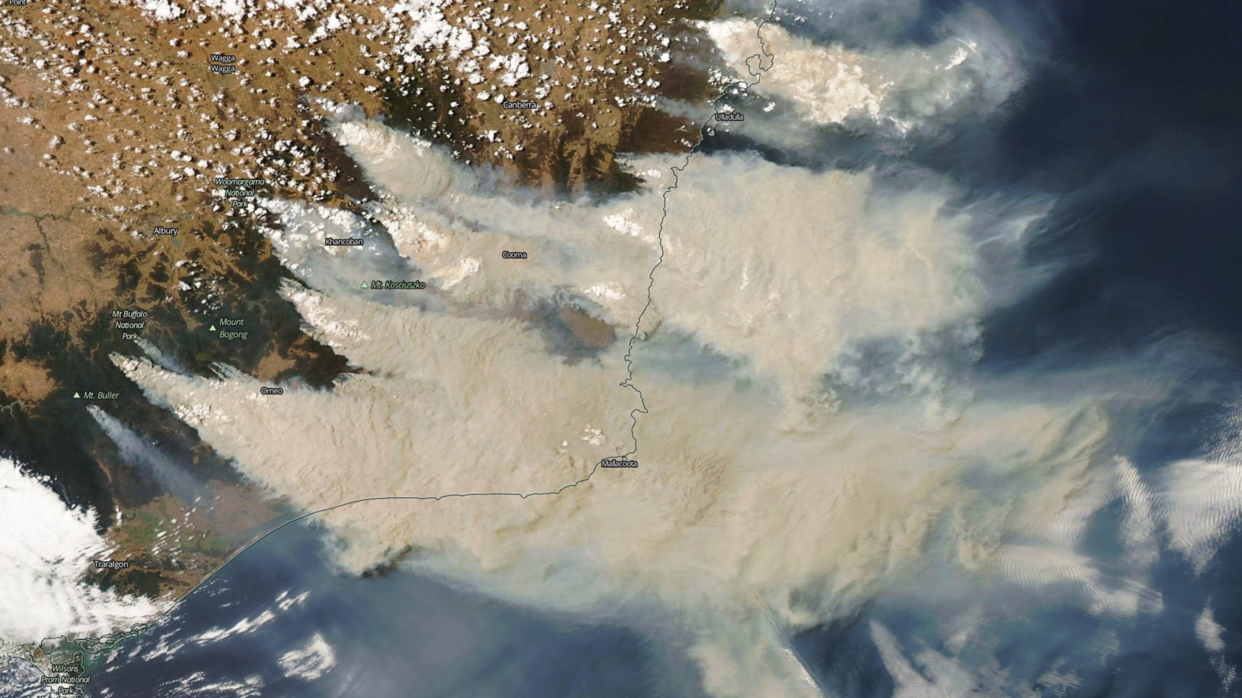
Smoke plumes from bushfires in southeast Australia on January 4, 2020, as seen by the MODIS imager on NASA’s Aqua satellite.
Summary Points
1) Global wildfire activity has decreased in recent decades, making any localized increase (or decrease) in wildfire activity difficult to attribute to ‘global climate change’.
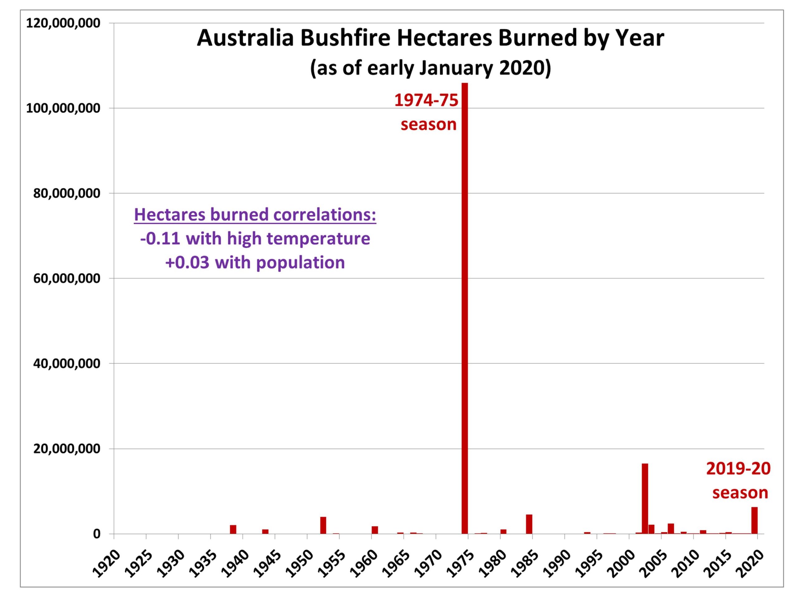
2) Like California, Australia is prone to bushfires every year during the dry season. Ample fuel and dry weather exists for devastating fires each year, even without excessive heat or drought, as illustrated by the record number of hectares burned (over 100 million) during 1974-75 when above-average precipitation and below-average temperatures existed.
3) Australian average temperatures in 2019 were well above what global warming theory can explain, illustrating the importance of natural year-to-year variability in weather patterns(e.g. drought and excessively high temperatures).
4) Australia precipitation was at a record low in 2019, but climate models predict no long-term trend in Australia precipitation, while the observed trend has been upward, not downward. This again highlights the importance of natural climate variability to fire weather conditions, as opposed to human-induced climate change.
5) While reductions in prescribed burning have probably contributed to the irregular increase in the number of years with large bush fires, a five-fold increase in population in the last 100 years has greatly increased potential ignition sources, both accidental and purposeful.
Historical Background
Australia has a long history of bush fires, with the Aborigines doing prescribed burns centuries (if not millennia) before European settlement. A good summary of the history of bushfires and their management was written by the CSIRO Division of Forestry twenty-five years ago, entitled Bushfires – An Integral Part of Australia’s Environment.
The current claim by many that human-caused climate change has made Australian bushfires worse is difficult to support, for a number of reasons. Bushfires (like wildfires elsewhere in the world) are a natural occurrence wherever there is strong seasonality in precipitation, with vegetation growing during the wet season and then becoming fuel for fire during the dry season.
All other factors being equal, wildfires (once ignited) will be made worse by higher temperatures, lower humidity, and stronger winds. But with the exception of dry lightning, the natural sources of fire ignition are pretty limited. High temperature and low humidity alone do not cause dead vegetation to spontaneously ignite.
As the human population increases, the potential ignition sources have increased rapidly. The population of Australia has increased five-fold in the last 100 years (from 5 million to 25 million). Discarded cigarettes and matches, vehicle catalytic converters, sparks from electrical equipment and transmission lines, campfires, prescribed burns going out of control, and arson are some of the more obvious source of human-caused ignition, and these can all be expected to increase with population.
Trends in Bushfire Activity
The following plot shows the major Australia bushfires over the same period of time (100 years) as the five-fold increase in the population of Australia. The data come from Wikipedia’s Bushfires in Australia.
Fig. 1. Yearly fire season (June through May) hectares burned by major bushfires in Australia since the 1919-20 season (2019-20 season total is as of January 7, 2020).
As can be seen, by far the largest area burned occurred during 1974-75, at over 100 million hectares (close to 15% of the total area of Australia). Curiously, though, according to Australia Bureau of Meteorology (BOM) data, the 1974-75 bushfires occurred during a year with above-average precipitation and below-average temperature. This is opposite to the narrative that major bushfires are a feature of just excessively hot and dry years.
Every dry season in Australia experiences excessive heat and low humidity.
Australia High Temperature Trends
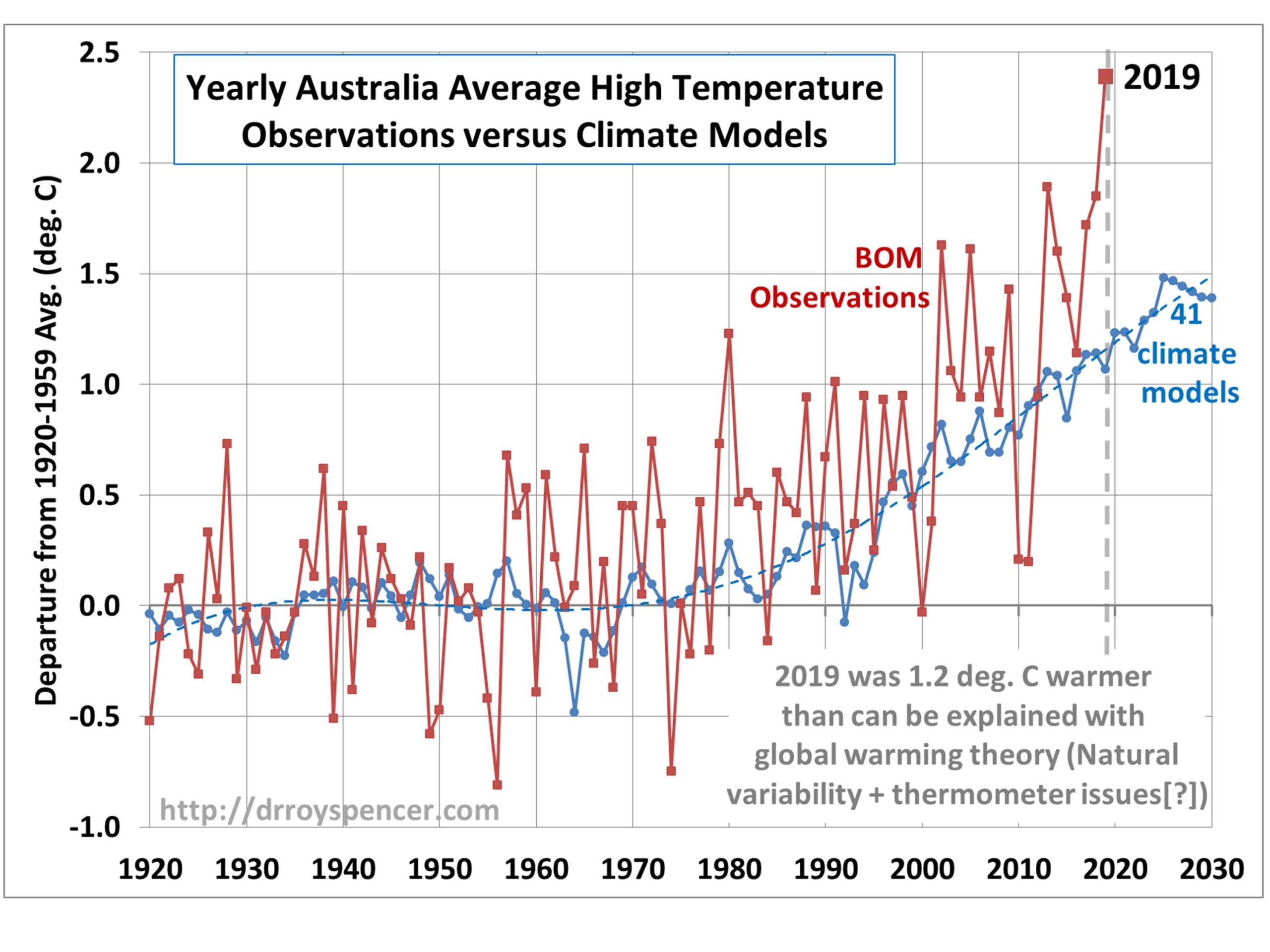
The following plot (in red) shows the yearly average variations in daily high temperature for Australia, compared to the 40-year average during 1920-1959.
Fig. 2. Yearly average high temperatures in Australia as estimated from thermometer data (red) and as simulated by the average of 41 climate models (blue). (Source).
Also shown in Fig. 2 (in blue) is the average of 41 CMIP5 climate models daily high temperature for Australia (from the KNMI Climate Explorer website). There are a few important points to be made from this plot.
First, if we correlate the yearly temperatures in Fig. 2 with the bushfire land area burned in Fig. 1, there is essentially no correlation (-0.11), primarily because of the huge 1974-75 event. If that year is removed from the data, there is a weak positive correlation (+0.19, barely significant at the 2-sigma level). But having statistics depend so much on single events (in this case, their removal from the dataset) is precisely one of the reasons why we should not use the current (2019-2020) wildfire events as an indicator of long-term climate change.
Secondly, while it is well known that the CMIP5 models are producing too much warming in the tropics compared to observations, in Australia just the opposite is happening: the BOM temperatures are showing more rapid warming than the average of the climate models produces. This could be a spurious result of changes in Australian thermometer measurement technology and data processing as has been claimed by Jennifer Marohasy.
Or, maybe the discrepancy is from natural climate variability. Who knows?
Finally, note the huge amount of year-to-year temperature variability in Fig. 2. Clearly, 2019 was exceptionally warm, but a good part of that warmth was likely due to natural variations in the tropics and subtropics, due to persistent El Nino conditions and associated changes in where precipitation regions versus clear air regions tend to get established in the tropics and subtropics.
Australia Precipitation Trends
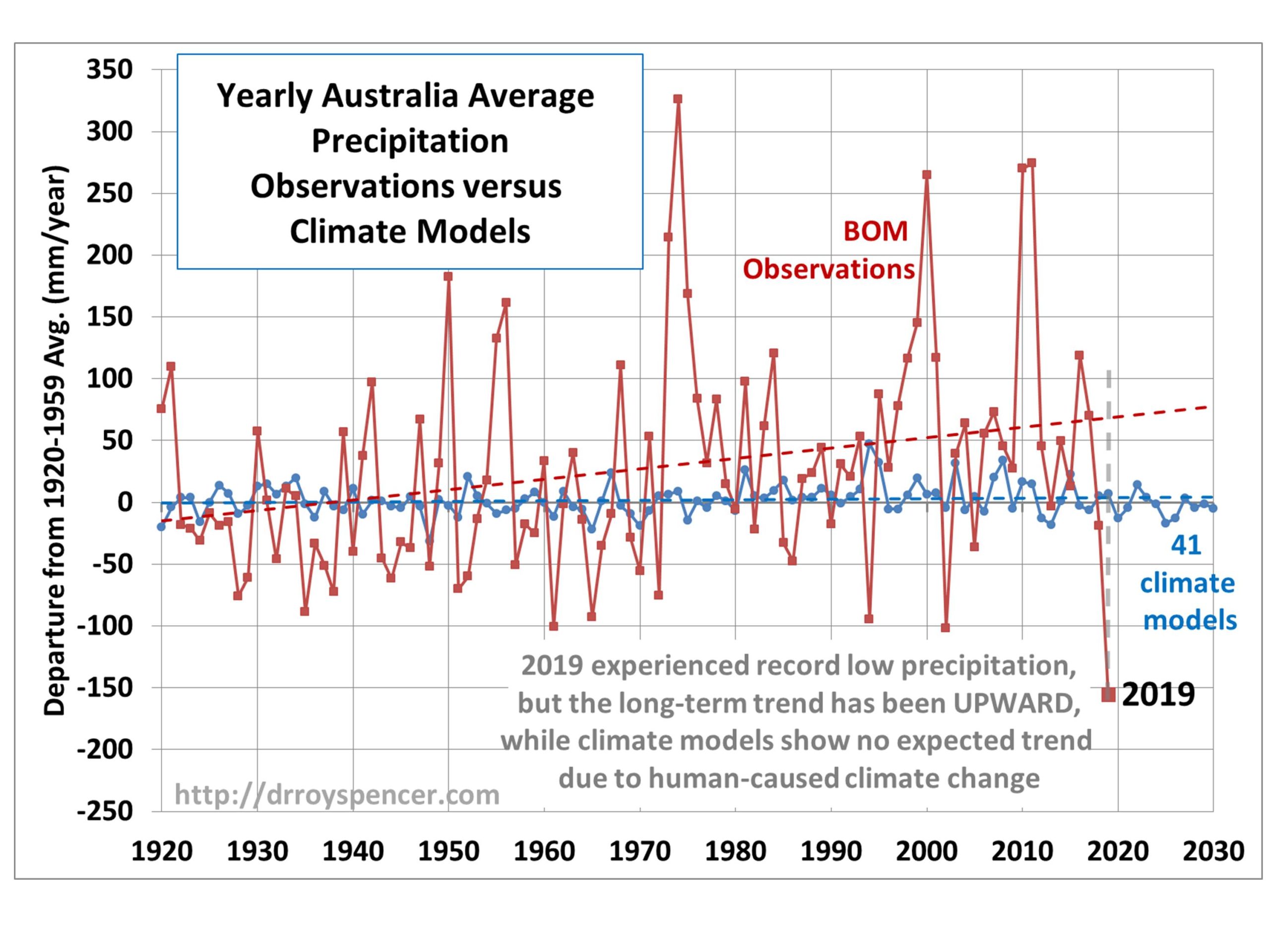
To drive home the point that any given year should not be used as evidence of a long-term trend, Australia precipitation provides an excellent example. The following plot is like the temperature plot above (Fig. 2), but now for precipitation as reported by the BOM (data here).
Fig. 3. As in Fig. 2, but for annual precipitation totals.
We can see that 2019 was definitely a dry year in Australia, right? Possibly a record-setter. But the long-term trend has been upward (not downward), again illustrating the fact that any given year might not have anything to do with the long-term trend, let alone human-induced climate change.
And regarding the latter, the blue curve in Fig. 3 shows that the expectation of global warming theory as embodied by the average of 41 climate models is that there should have been no long-term trend in Australia precipitation, despite claims by the media, pseudo-experts, and Hollywood celebrities to the contrary.
It should be kept in mind that wildfire risk can actually increase with more precipitation during the growing season preceding fire season. More precipitation produces more fuel. In fact, there is a positive correlation between the precipitation data in Fig. 3 and bushfire hectares burned (+0.30, significant at the 3-sigma level). Now, I am not claiming that hot, dry conditions do not favor more bushfire activity. They indeed do (during fire season), everything else being the same. But the current 2019-2020 increase in bushfires would be difficult to tie to global warming theory based upon the evidence in the above three plots.
Global Wildfire Activity
If human-caused climate change (or even natural climate change) was causing wildfire activity to increase, it should show up much better in global statistics than in any specific region, like Australia. Of course any specific region can have an upward (or downward) trend in wildfire activity, simply because of the natural, chaotic variations in weather and climate.
But, contrary to popular perception, a global survey of wildfire activity has found that recent decades have actually experienced less fire activity (Doerr & Santin, 2016), not more. This means there are more areas experiencing a decrease in wildfire activity than there are areas experiencing more wildfires.
Why isn’t this decrease being attributed to human-caused climate change?
Concluding Comments
There are multiple reasons why people have the impression that wildfires are getting worse and human-caused climate change is to blame. First, the news tends to report only disasters… not a lack of disasters. The desire for more clicks means that headlines are increasingly sensationalized. The media can always find at least one expert to support the desired narrative.
Second, the spread of news is now rapid and it penetrates deeply, being spread through social media.
Third, an increasing number of environmental advocacy groups seize upon any natural disaster and declare it to be caused by increasing CO2 in the atmosphere. The hyperbolic and counter-factual claims of Extinction Rebellion is one of the best recent examples of this.
This is all against a backdrop of government funded science that receives funding in direct proportion to the threat to life and property that the researcher can claim exists if science answers are not found, and policy is not changed. So, it should come at no surprise that there is political influence on what research gets funding when the outcome of that research directly affects public policy.
My personal opinion, based upon the available evidence, is that any long-term increase in wildfire activity in any specific location like Australia (or California) is dominated by the increase in human-caused ignition events, whether they be accidental or purposeful. A related reason is the increasing pressure by the public to reduce prescribed burns, clearing of dead vegetation, and cutting of fire breaks, which the public believes to have short term benefits to beauty and wildlife preservation, but results in long term consequences that are just the opposite and much worse.
Recent news reports claim that dozens of people have been arrested in Australia on arson charges, a phenomenon which we must assume has also increased by at least five-fold (like population) in the last 100 years. Accidental sources of ignition also increase in lockstep with the increasing population and all of the infrastructure that comes along with more people (vehicles, power lines, campfires, discarded matches and cigarettes, etc.)
So, to automatically blame the Australian bushfires on human-caused climate change is mostly alarmist nonsense, with virtually no basis in fact.
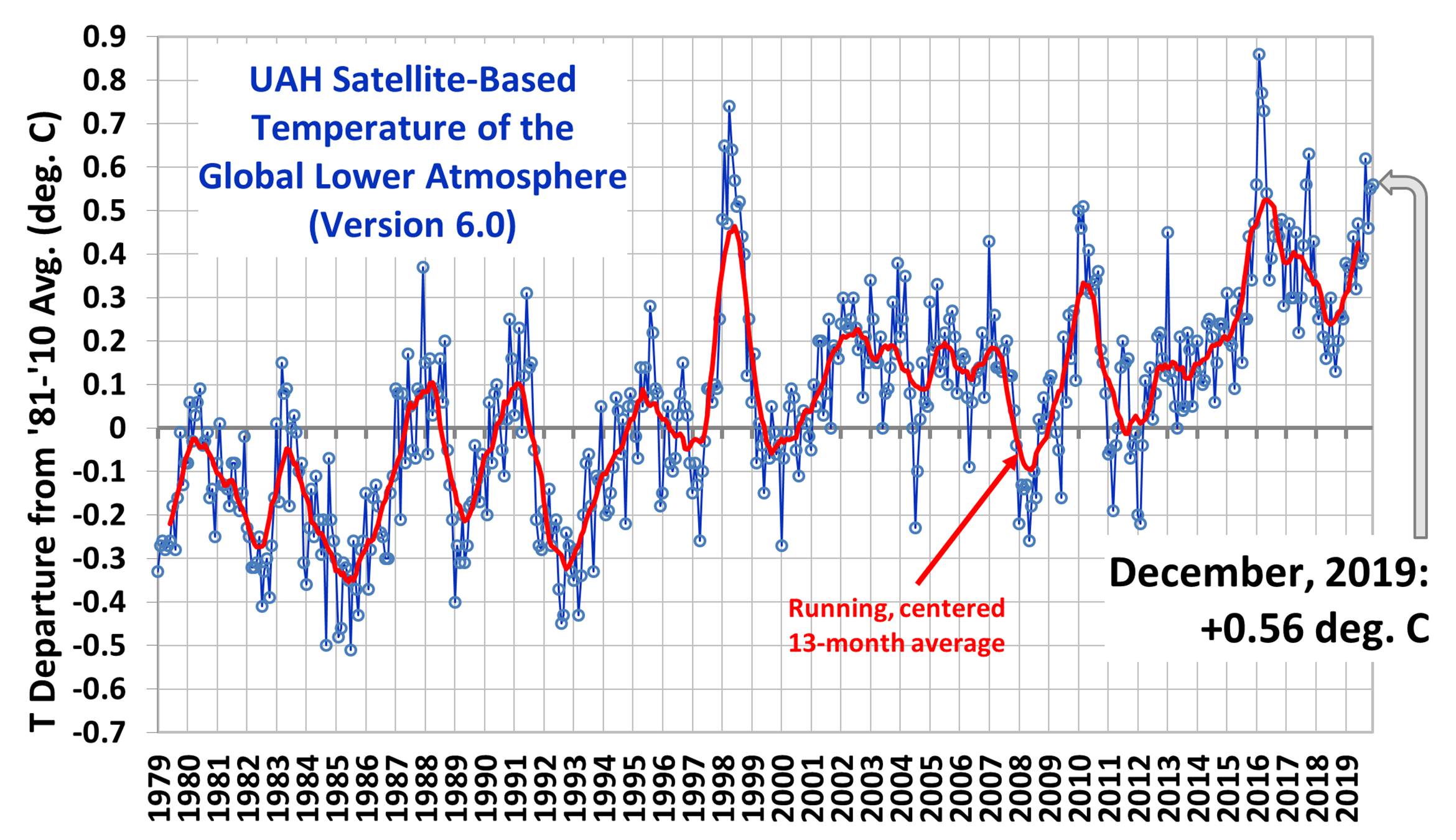
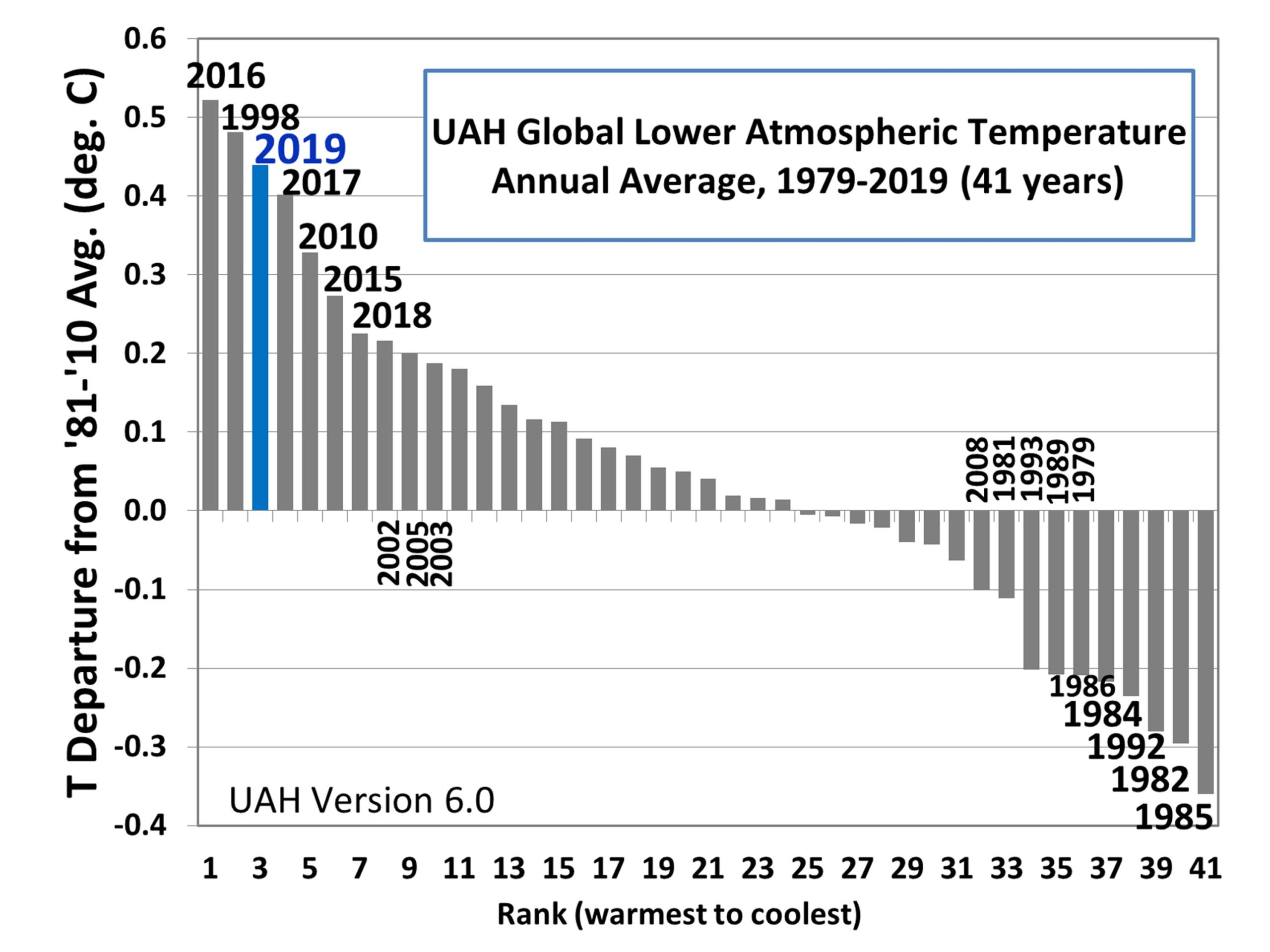
2019 was the third warmest year (+0.44 deg. C) in the 41 year satellite record, after 2016 (+0.52 deg. C) and 1998 (+0.48 deg. C).
The Version 6.0 global average lower tropospheric temperature (LT) anomaly for December, 2019 was +0.56 deg. C, statistically unchanged from the November value of +0.55 deg. C.
The yearly rankings over the 41-year satellite-based temperature record shows 2019 as the third warmest, behind 2016 and 1998.
The linear warming trend since January, 1979 remains at +0.13 C/decade (+0.11 C/decade over the global-averaged oceans, and +0.18 C/decade over global-averaged land).
Various regional LT departures from the 30-year (1981-2010) average for the last 24 months are:
The UAH LT global anomaly image for December, 2019 should be available in the next few days here.
The global and regional monthly anomalies for the various atmospheric layers we monitor should be available in the next few days at the following locations:
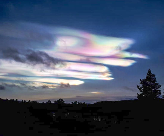
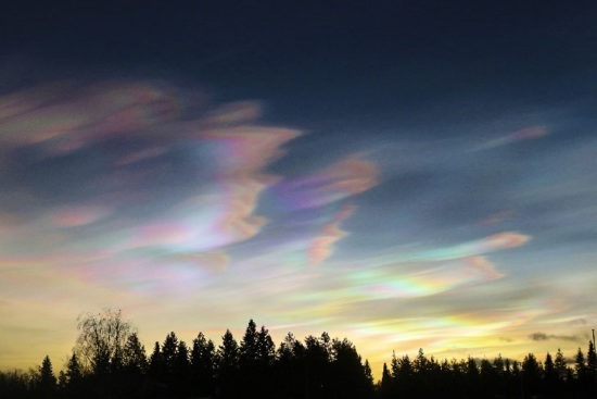
Polar Stratospheric Cloud display (smartphone photo posted by Reddit user Breuuan on Dec. 31, 2019.)
Increasing carbon dioxide in the atmosphere will continue to cause upper atmospheric cooling in the 2020s, which will lead to some of the most beautiful cloud displays ever witnessed by human eyes.
Along with the warming in the lower atmosphere that more CO2 is theoretically expected to produce, the upper atmosphere is supposed to cool even more strongly. For example, in our satellite observations since 1979, we have observed about 3-4 times as much cooling in the middle stratosphere as warming in the troposphere over the last four decades. This cooling is expected to exist even higher up, into the upper mesosphere and beyond, which is at the edge of outer space and where meteors burn up. The current record solar minimum conditions are probably also contributing to this cooling.
Polar Stratospheric Clouds and Noctilucent Clouds are Increasing
As 2019 came to a close, reports of some of the most vivid opalescent displays of wintertime polar stratospheric clouds (PSCs) in memory have been coming in from Northern Europe. These clouds require very cold temperatures in the stratosphere (-80 deg. C or colder). They show up shortly after sunset or before sunrise when the sun is still shining at that high altitude (15-25 km), while the usual weather-related clouds in the troposphere are no longer illuminated by the sun.
Wintertime polar stratospheric clouds in Sweden, Dec 30, 2019 (by Patricia Cowern Israelsson).
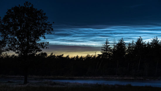
In the summertime in the polar regions, electric-blue noctilucent clouds (NLCs) are sometimes seen in the upper mesosphere (80-85 km) where temperatures plunge to the coldest anywhere on Earth, -100 deg. C. Like PSCs, they are seen after sunset or before sunrise, but due to their great altitude occur when the sun is well below the horizon and some brighter stars are beginning to shine. These clouds exist at literally the edge of space, above 99.999% of the mass of the atmosphere, and are believed to be seeded by meteoric dust.
These clouds have a rippled appearance, and time lapse photography has revealed an amazing variety of undulations, like waves from multiple pebbles thrown in a pond interacting. The following 4K time lapse video shows cloud behavior unlike any you have seen before, and is well worth the 2 minutes it takes to watch (go full-screen):
Last year (2019) NLCs were observed well outside the polar regions for the first time in recorded history, as far south as southern California and Nevada. This is due to some combination of colder temperatures and higher water vapor amounts (methane is converted to water vapor at these altitudes, and increasing atmospheric methane could be causing higher humidity up there).

 Home/Blog