The continuing global-average warmth over the last year has caused a few people to ask for my opinion regarding potential explanations. So, I updated the 1D energy budget model I described a couple years ago here with the most recent Multivariate ENSO Index (MEIv2) data. The model is initialized in the year 1765, has two ocean layers, and is forced with the RCP6 radiative forcing scenario and the history of El Nino and La Nina activity since the late 1800s.
The result shows that the global-average (60N-60S) ocean sea surface temperature (SST) data in recent months are well explained as a reflection of continuing weak El Nino conditions, on top of a long-term warming trend.

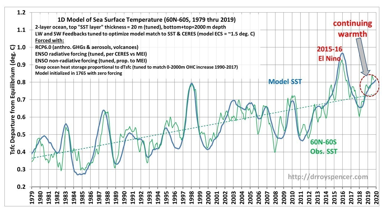
The model is described in more detail below, but here I have optimized the feedbacks and rate of deep ocean heat storage to match the 41-year warming trend during 1979-2019 and increase in 0-2000m ocean heat content during 1990-2017.
While the existence of a warming trend in the current model is due to increasing CO2 (I use the RCP6 radiative forcing scenario), I agree that natural climate variability is also a possibility, or (in my opinion) some combination of the two. The rate of deep-ocean heat storage since 1990 (see Fig. 3, below) represents only 1 part in 330 of global energy flows in and out of the climate system, and no one knows whether there exists a natural energy balance to that level of accuracy. The IPCC simply *assumes* it exists, and then concludes long-term warming must be due to increasing CO2. The year-to-year fluctuations are mostly the result of the El Nino/La Nina activity as reflected in the MEI index data, plus the 1982 (El Chichon) and 1991 (Pinatubo) major volcanic eruptions.
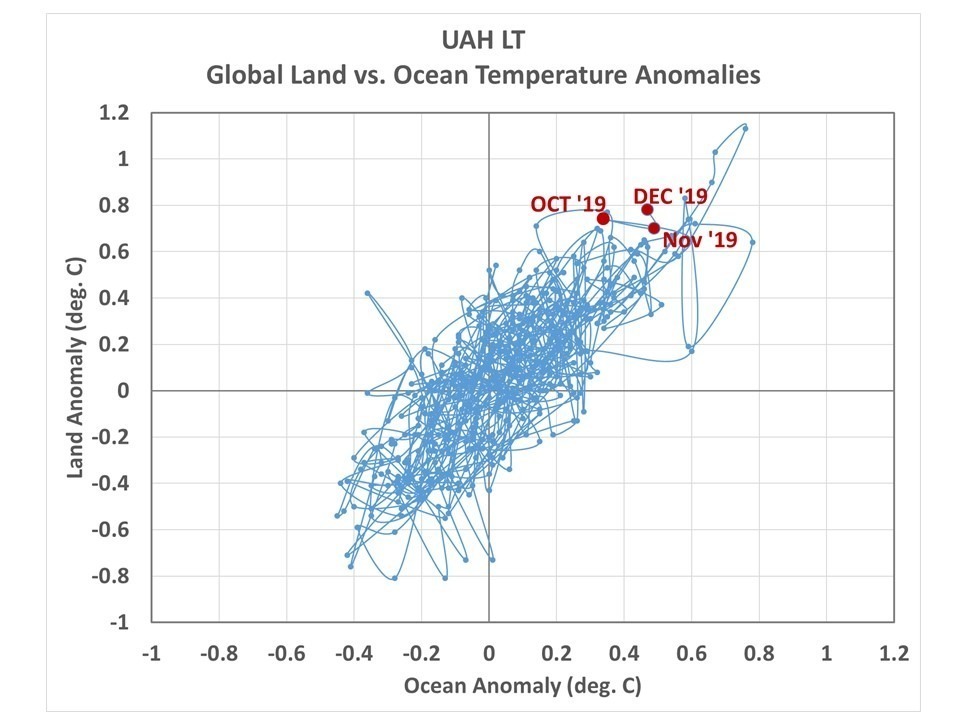
When I showed this to John Christy, he asked whether the land temperatures have been unusually warm compared to the ocean temperatures (the model only explains ocean temperatures). The following plot shows that for our UAH lower tropospheric (LT) temperature product, the last three months of 2019 are in pretty good agreement with the rest of the post-1979 record, with land typically warming (and cooling) more than the ocean, as would be expected for the difference in heat capacities, and recent months not falling outside that general envelope. The same is true of the surface data (not shown) which I have only through October 2019.

The model performance since 1900 is shown next, along with the fit of the model deep-ocean temperatures to observations since 1990. Note that the warming leading up to the 1940s is captured, which in the model is due to stronger El Nino activity during that time.

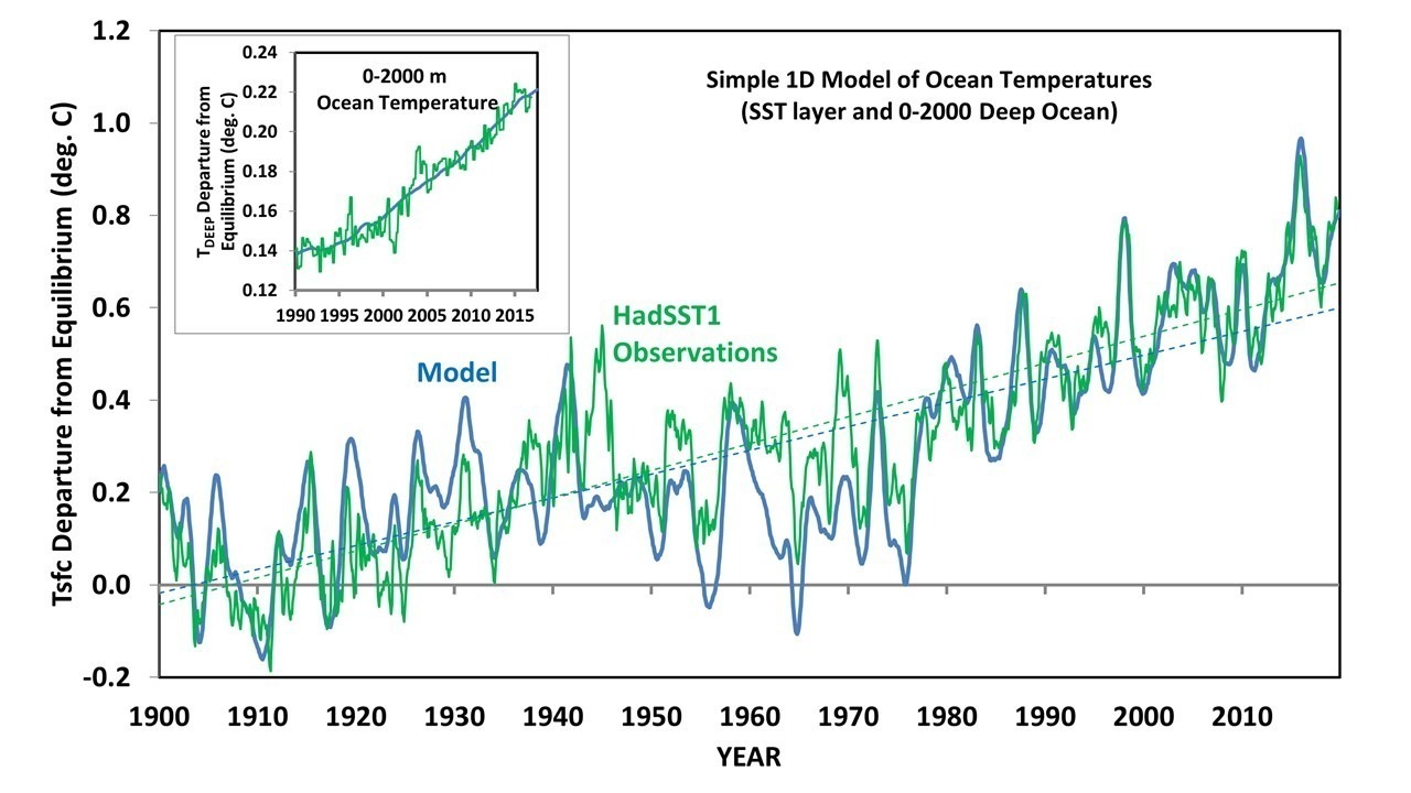
The model equilibrium climate sensitivity which provides the best match to the observational data is only 1.54 deg. C, using HadSST1 data. If I use HadSST3 data, the ECS increases to 1.7 deg. C, but the model temperature trends 1880-2019 and 1979-2019 can no longer be made to closely approximate the observations. This suggests that the HadSST1 dataset might be a more accurate record than HadSST3 for multi-decadal temperature variability, although I’m sure other explanations could be envisioned (e.g. errors in the RCP6 radiative forcing, especially from aerosol pollution).
A Brief Review of the 1D Model
The model is not just a simple statistical fit of observed temperatures to RCP6 and El Nino/La Nina data. Instead, it uses the energy budget equation to compute the monthly change in temperature of ocean near-surface layer due to changes in radiative forcing, radiative feedback, and deep-ocean heat storage. As such, each model time step influences the next model time step, which means the model adjustable parameters cannot be optimized by simple statistical regression techniques. Instead, changes are manually made to the adjustable model parameters, the model is run, and then compared to a variety of observations (SST, deep ocean temperatures, and how CERES radiative fluxes vary with the MEI index). Many combinations of model adjustable parameters will give a reasonably good fit to the data, but only within certain bounds.
There are a total of seven adjustable parameters in the model, and five time-dependent datasets whose behavior is explained with various levels of success by the model (HadSST, NODC 0-2000m deep ocean temperature [1990-2017], and the lag-regression coefficients of MEI versus CERES satellite SW, LW, and Net radiative fluxes [March 2000 through April 2019]).
The model is initialized in 1765 (when the RCP6 radiative forcing dataset begins) which is also when the climate system is (for simplicity) assumed to be in energy balance. Given the existence of the Little Ice Age, I realize this is a dubious assumption.
The energy budget model computes the monthly change in temperature (dT/dt) due to the RCP6 radiative forcing scenario (which starts in 1765, W/m2) and the observed history of El Nino and La Nina activity (starting in 1880 from the extended MEI index, intercalibrated with and updated to the present with the newer MEIv2 dataset (W/m2 per MEI value, with a constant of proportionality that is consistent with CERES satellite observations since 2000). As I have discussed before, from CERES satellite radiative budget data we know that El Nino is preceded by energy accumulation in the climate system, mainly increasing solar input from reduced cloudiness, while La Nina experiences the opposite. I use the average of the MEI value in several months after current model time dT/dt computation, which seems to provide good time phasing of the model with the observations.
Also, an energy conserving non-radiative forcing term is included, proportional to MEI at zero time lag, which represents the change in upwelling during El Nino and La Nina, with (for example) top layer warming and deep ocean cooling during El Nino.
A top ocean layer assumed to represent SST is adjusted to maximize agreement with observations for short-term variability, and as the ocean warms above the assumed energy equilibrium value, heat is pumped into the deep ocean (2,000 m depth) at a rate that is adjusted to match recent warming of the deep ocean.
Empirically-adjusted longwave IR and shortwave solar feedback parameters represent how much extra energy is lost to outer space as the system warms. These are adjusted to provide reasonable agreement with CERES-vs.-MEI data during 2000-2019, which are a combination of both forcing and feedback related to El Nino and La Nina.
Generally speaking, changing any one of the adjustable parameters requires changes in one or more of the other parameters in order for the model to remain reasonably close to the variety of observations. There is no one “best” set of parameter choices which gives optimum agreement to the observations. All reasonable choices produce equilibrium climate sensitivities in the range of 1.4 to 1.7 deg. C.
Pretty impressive results from just three basic forcings!
What is the mechanism in the 1940’s to 70’s hiatus?
Stop talking to yourself people will think you’re crazy
Good point Eben!
Still interesting, all the rise explained by RCP6 forcings.
Occam wins again.
With due respect to our host, you are not correct: there are more than three inputs here. Dr Spencer is very clear about all the tuning factors. It’s von Neuman’s elephant all over again. Given enough inputs and enough free variables to tune you can match just about anything.
since one of the inputs in an SST related metric, to some extent it explains SST with SST.
Here is the real problem with this analysis:
“which are departures from assumed energy equilibrium in 1765.”
What is a little worrying here is that Dr. Spencer seems to be buckling to the concensus pressure. There is no valid reason to assume the climate was in equilibrium in 1765. It was only just coming out of the LIA. That implicitly accepts the unsubstantiated premise that any long term warming since that time must be attributable to AGW.
Sadly, that is just kowtowing to the climate scammers.
Which is why I admitted in the article that assuming energy equilibrium in 1765 was a “dubious assumption” because of the Little Ice Age. Assumptions are necessary in any physical model in order to get an answer. You learn something in the process. -Roy
From the link:
“Key features of composite positive MEI events (warm, El Nio) include (1) anomalously warm SSTs across the east-central equatorial Pacific, (2) anomalously high SLP over Indonesia and the western tropical Pacific and low SLP over the eastern tropical Pacific, (3) reduction or reversal of tropical Pacific easterly winds (trade winds), (4) suppressed tropical convection (positive OLR) over Indonesia and Western Pacific and enhanced convection (negative OLR) over the central Pacific.”
The only “SST related metric” is comparing equatorial Pacific SST to global SST. If the ENSO didn’t affect global sea temps the model would not work. Same for RCP6.0 forcings. Using established science is not “kowtowing to the climate scammers”.
“What is a little worrying here is that Dr. Spencer seems to be buckling to the concensus pressure. There is no valid reason to assume the climate was in equilibrium in 1765. It was only just coming out of the LIA. That implicitly accepts the unsubstantiated premise that any long term warming since that time must be attributable to AGW.”
Greg, he is simply testing a hypothesis that a few known effects can explain the temperature record.
How is that buckling to pressure? He is simply doing what science is supposed to do.
“Greg, he is simply testing a hypothesis that a few known effects can explain the temperature record.”
The key hypothesis is that the ASSUMPTION climate was in equilibrium until we came along and messed it up.
” If the ENSO didn’t affect global sea temps the model would not work.”
There is correlation with Pacific ocean metrics since it covers half the globe. That means it helps explain the wiggles.
I think what our host is trying to do here is kind of go along with the alarmist reasoning and still demonstrate that this leads to less ECS than they claim using failed models.
However, that is a dangerous path to follow since it is half way to acceptance. Maybe he should have stated it more like :
let’s for the sake of argument make the totally unfounded and improbably assumption that the climate was in equilibrium and that any longer term trend can be attributed to AGW and see what ECS this leads to.
“I think what our host is trying to do here is kind of go along with the alarmist reasoning and still demonstrate that this leads to less ECS than they claim using failed models.
Our host agrees that greenhouse gasses warm the planet, he just doesn’t believe it will lead to catastrophic climate change. This is something he’s made clear on this site.
“I think what our host is trying to do here is kind of go along with the alarmist reasoning..”
“However, that is a dangerous path to follow since it is half way to acceptance”
I see, you are saying that real skeptic scientists should not test hypotheses and follow evidence..that would be dangerous.
Instead they should only be following a party line skeptical narrative?
The causes of the temp record changes we have need to be explained.
The LIA is a feature of the record, not a cause.
Certainly a nice fit.
I dont understand the “The rate of deep-ocean heat storage since 1990 (see Fig. 3, below) represents only 1 part in 330 of global energy flows in and out of the climate system”
because I thought it was ~ 0.7 W/m^2 recently? And your figure 3 inset seems to give ~ 0.5 W/m^2 since 1990.
Sorry, I get it now. Energy flows are like 240 W/m^2.
Nice work! It would be interesting to see what the solar-cycle forcing according to the mechanism proposed by Svensmark / Shaviv would give with your model. What would the resulting ECS be then and how good agreement would it provide to the datasets that you describe? As I understand it, the model result is currently given under the assumption that CO2 radiative forcing is the main (only?) factor causing the long term increase in temperature.
All climate models have so far matched the past but failed future projection using radiative forcing. Will this be any different using the same concept?
Without a way to predict the ENSO cycle future models can’t be this accurate. The MEI.v2 from 1979 to 2019 averages out to 0.014 so over time the ENSO effects cancel out. The model should work at the 30 – 40 year scale.
Roy,
A question on which climate sensitivity is appropriate to use here: Transient Climate Response or Equilibrium Climate Sensitivity?
TCR is the response to forcing at the time of forcing (a little more complicated than that, but that’s the basic idea).
ECR is the response after the system equilibrates with the forcing, so the response of thr system lags the forcing.
It seems that your results are based on response at the time of forcing, but I’m not sure. Would TCR be more appropriate?
AR5 TCR is 1.8 C (+/- 0.6)
The model uses feedback parameters, which determine ECS, not TCR. If I was to keep the RCP6 net forcing constant after 2019, then the model would equilibrate to about 1.5 deg. C warmer than in 1765 after a long period of time, say 100-200 years.
‘net forcing constant after 2019’ but then the co2 is not doubling but staying constant at 415 ppm?
Then your 1.5 C is not then a result of 2x preindustrial co2, the usual climate sensitivity.
???
Roy,
“The model uses feedback parameters, which determine ECS, not TCR.”
No, TCR includes feedbacks, and is different from ECS mainly in that it is an estimate of response “at the time of doubling,” rather than of the response after some time has passed to allow most of the equilibration to occur.
IPCC says:
Transient climate response
The change in the global mean surface temperature, averaged over a 20-year period, centered at the time of atmospheric CO2 doubling, in a climate model simulation in which CO2 increases at 1% yr-1 from pre-industrial. It is a measure of the strength of climate feedbacks and the timescale of ocean heat uptake.
https://www.ipcc.ch/sr15/chapter/glossary/
If you are gauging climate sensitivity from response-at-the-time – even with feedbacks – then your results are more an estimate of TCR than ECS. If letting the model run on as you suggest gives a further 1.5C response, then it appears the estimate of ECS is about 3C.
The best past model prediction yet
Hi Eben, this one is even better:
https://www.carbonbrief.org/guest-post-why-natural-cycles-only-play-small-role-in-rate-of-global-warming
Hi Roy,
Would you like to comment on this article if you have time:
“Some say we’ve seen Australia’s bushfires worse than this, but they’re ignoring a few facts”
https://www.stuff.co.nz/world/australia/118770134/some-say-weve-seen-australias-bushfires-worse-than-this-but-theyre-ignoring-a-few-facts?cid=app-iPad
Regards John
I’ve been trying to take a dispassionate look at the recent bushfires, extreme weather events and climate, and I think the article does very well at summing things up.
One thing is annoying – most articles like this point to the lowest or near-lowest rainfall in the region during 2019, in the same sentence or next as mentioning the record high temps for 2019. Then the upward temeprature trend is mentioned – but NOT that the trend for rainfall is generally upwards or flat.
In these articles, I would prefer to see that mentioned and dealt with, but it gets in the way of the narrative, apparently.
IMO, the warming temp trend over time must influence bush fires. It’s basic physics. The higher the temperature, the less difference between ambient air temp and the combustion point of natural fuels.
Many of the purported links between climate and the severity of these bushfires are tenuous, as far as I can read, but not regarding the increase in temperature. Another increased trend is the Forest Fire Danger Index, which assesses bushfire potential on a range of factors.
The article gets right that the CSIRO predicted greater risk of intense bush fires – but it doesn’t go far enough. I’ve read through quite a few predictive reports from CSIRO and other bodies commissioned by successive governments, as well as research papers on Austraslian bushfires. There are reports from the 2000s that predicted the increase in FFDI quite accurately to 2020.
Does CO2 or climate change cause bush fires? No. But at least with respect to ttemperature, AGW is making bushfires worse in general, though it will be different depending which part of Australia. The North is meant to get wetter in the future, so that may mitigate warmer temps re bushfires.
There might be worse to come, regarding Australian droughts, but not necessarily caused by human emissions of CO2.
Ice core analyses from Law Dome in Antarctica have provided a 1,000 year history of droughts in Australia.
https://www.researchgate.net/publication/291167238_A_new_direction_for_Antarctic_ice_cores_reconstructing_Pacific_decadal_variability_and_Australian_drought_history_from_the_Law_Dome_ice_core
“Eight ‘mega-droughts’ (dry periods >5 years duration) were identified over the last millennium. Six mega-droughts occurred between AD 1000-1320 including one 39 y drought (AD 1174–1212). Water resources and infrastructure planning in Australia has been based on very limited statistical certainty around drought risk due to the short ( 100 year) instrumental record and lack of rainfall proxies. This study shows that, similar to SW North America, Australia also experienced mega-droughts during the medieval period. Knowledge of the occurrence, duration and frequency of such mega-droughts will greatly improve drought risk assessment in Australia.”
It’s possible Australia could experience another 39-year drought in the future which might be unrelated to the minuscule amounts of CO2 in the atmosphere, or at least insignificantly related.
In order to believe the global warming and man made bad weather nonsense you must never look further back than 150 years
The agricultural revolution altered global temperatures as much as the industrial revolution.
https://tinyurl.com/rhzabrw
‘Six mega-droughts occurred between AD 1000-1320 including one 39 y drought (AD 1174–1212).’
Given that those were during the MWP, a warmer period, but most likely less warm than the 21st century, this is not very comforting..
That’s right. It’s not meant to be comforting. However, the delusion that we can prevent such extreme weather events simply by reducing our CO2 emissions, is very comforting.
Heh, classic straw man there. Few, if any, think that CO2 causes weather, extreme or otherwise.
That does not follow, Vincent.
IF megadroughts are correlated with global warm periods, then AGW should be a concern and limited.
This drought killed between 30 to 60 million people till 1878:
https://blogs.ei.columbia.edu/2017/12/15/causes-great-famine-drought/
Nate says:
January 15, 2020 at 9:36 PM
“That does not follow, Vincent.
IF megadroughts are correlated with global warm periods, then AGW should be a concern and limited.”
—————————————————————–
Nate,
Extreme weather events should always be a concern whether the climate is warming or cooling. Assuming that reducing human-caused CO2 emissions will fix the problem could be the biggest disaster of all.
http://www.drroyspencer.com/2020/01/weak-el-nino-conditions-help-explain-recent-global-warmth/#comment-423438
barry
Somewhere upthread, you wrote a propos bushfires:
IMO, the warming temp trend over time must influence bush fires. It’s basic physics. The higher the temperature, the less difference between ambient air temp and the combustion point of natural fuels.
If I well remember, you are an Australian, while I look at these terrifying events from my far, “upabove” Germany.
I had a look at may online articles and blog comments, e.g. WUWT, Tamino and here.
Of course, there is clearly a warming trend, even if you restrict the station set to NSW, Canberra and Victoria:
https://drive.google.com/file/d/1oC13owo5AeumsX8YHaIbGhsJuko2bp-g/view
And that is in the subjective viewer’s opinion the primary reason why the 2019 season was so harsh in comparison with the recent seasons of that kind: 2009, 1974, 1939.
1974 was eliminated due to a severe bias of not accounting for the huge amount of savanna fires in that year.
But when you look at a day-by-day comparison between the three other years, you see this:
https://drive.google.com/file/d/1O1jKHHMvT3VKyN58uzTFZjW3vtAkoWwC/view
We clearly see that these years do not differ very much in their daily behavior.
How do you explain that?
Well, I have some questions.
I can’t remember if the GHCN daily set is raw or homogenised, or if the data they gather from Australia is raw or based on the ACORN dataset. Do you know? Because that could make a significant difference if the regions are small enough.
Also, you’ve labeled the chart NSW, Victoria and Canberra. The first 2 are states, the latter is a city. Have you weighted the Canberra record equally (one third of the average) against the 2 states?
If the data is raw and Canberra is given large weighting, then the resulting temperature graphs could be contaminated with respect to climate.
I reccomend using the ACORN dataset, as do the BoM here. As you probably know, you can plot on a web page quite interesting details of Australian climate over time. You can find warmer months in the past, depending on location and the month you choose, but annual temps have recent years as the warmest in NSW/ACT and VIC.
To answer under an assumption: if the data you used was excellent quality and the spatial selection was a good representation of regional climate, then we would have trouble claiming that the warmth of 2019 is anything special in terms of climate and bush fires in Australia.
barry
1. “I can’t remember if the GHCN daily set is raw or homogenised, or if the data they gather from Australia is raw or based on the ACORN dataset.”
GHCN daily is the rawest data set known to me. It even contains, for many today’s records in the US – especially in AK – and in very old Australian records, errors due to sudden so-called Celsius-Fahrenheit bumps (i.e. within which Fahrenheit temperatures are/were transmitted as Celsius).
barry, I obtained from BoM a few days ago new links to ACORN V2 data, and all that looks very, very homogenised in comparison with GHCN daily. What they do is similar to GHCN V4 adjusted (which contains, unlike GHCN V3 adjusted, homogenised structures).
I’ll upload a comparison of them when I have some time to do.
*
2. “… then we would have trouble claiming that the warmth of 2019 is anything special in terms of climate and bush fires in Australia.”
I agree.
That is exactly the reason why FDDI is so important: it measures much more than warmth only – just like MEI measures much more than SSTs in the small Nino3+4 area (5N-5S–170W-120W).
barry
“Also, youve labeled the chart NSW, Victoria and Canberra. The first 2 are states, the latter is a city. Have you weighted the Canberra record equally (one third of the average) against the 2 states?”
There was no weighting of any kind. I collected all GHCN daily stations found in these three territories (with ‘Canberra’ I meant in fact the Australian Capital Territory, not the city) and built the gridded average of their anomalies.
Here you see the list of all these 644 stations (ACORN V2 is based on 112 stations for the entire Australia):
https://drive.google.com/file/d/1GZRhqoTTM7LfylZsrLwNG5S3cPr_QCuw/view
Of course: not all of them were used for anomaly computing, as some had no sufficient data for the 1981-2010 period, nor did their surrounding grid cell either.
68 were rejected, giving 576 for the entire period starting in 1855; only 13 were active in 1906, 23 in 1939, 320 in 1974, 276 in 2009, and 233 in 2019.
Here is, as an info without great relevance, the top10 of the daily maxima recorded during the generation of the time series:
ASN00076077 ___MILDURA_POST_OFFICE________ 1906 1 7 50.7 (C)
ASN00076077 ___MILDURA_POST_OFFICE________ 1906 1 6 50.1
ASN00078077 ___WARRACKNABEAL_MUSEUM_______ 2018 1 19 50.0
ASN00048013 ___BOURKE_POST_OFFICE_________ 1903 1 4 49.7
ASN00076077 ___MILDURA_POST_OFFICE________ 1906 1 24 49.4
ASN00076077 ___MILDURA_POST_OFFICE________ 1904 12 31 49.4
ASN00052026 ___WALGETT_COUNCIL_DEPOT______ 1903 1 3 49.2
ASN00052088 ___WALGETT_AIRPORT_AWS________ 2014 1 3 49.1
ASN00084142 ___GELANTIPY__________________ 2019 12 30 48.9
ASN00076077 ___MILDURA_POST_OFFICE________ 1905 1 1 48.9
A warmista would cry ‘Oh look, look! 2018 and 2019 in the top 10!’
This is of course pure nonsense. To have a fair comparison, you must calculate, for all the years you want to look at, the average daily maximum found in e.g. the top 1000 measurements.
2019: 166 days, 46.5 C on average
2009: 61 / 46.5 C
1939: 32 / 46.6 C
1906: 21 / 47.4 C
1974 does not appear until you extend the top window up to 100,000 daily measurements.
“That is exactly the reason why FDDI is so important”
Agreed. Here is an anomaly map of FFDI changes since 1978.
https://www.abc.net.au/news/2019-11-13/ffdi-change-from-1978-to-2017/11699560
Here is a paper on FFDI from 1973
https://journals.plos.org/plosone/article?id=10.1371/journal.pone.0222328
And a paper predicting changes to FFDI by the CSIRO (interestingly, 2020 is one of the key dates).
http://www.cmar.csiro.au/e-print/open/hennessykj_2005b.pdf
I’ve read the last one, skimmed the former and have read a few articles and government reports as well. My provisional opinion, for what it’s worth, is that of all the indicators, temperature is the one that has the clearest signal (ACORN data) – perhaps the only one with a clear signal – and is the only driver that can be reasonably linked to any changes in bush fire intensity, seasonal start date, kinds of areas burned, and duration.
Meant to link to the BoM in the last post.
https://tinyurl.com/uywm28f
Looking at the graph of the Annual maximum temperature anomaly in Victoria from 1910 to 2019, it seems that the cooling period between 1940 and 1958 (approximately) is almost as significant as the warming between 1996 to 2019 (approximately).
I can’t make sense of the black line which is presumably representing a trend.
Vincent
“… it seems that the cooling period between 1940 and 1958 (approximately)…”
Oh la la… on croit lire ici la prose d’un sosie de Robertson.
Jesus, Vincent.
The Vic anomalies between 1940 and 1960 were drawn in blue because they are BELOW the baseline represented by the mean of 1961-1990, and NOT because they represent any cooling!
Cooling is – independently of above or below that baseline – represented by anomalies declining from left to right, and not by color.
And that you don’t understand this simple matter perfectly explains why you write:
“I cant make sense of the black line which is presumably representing a trend.”
Yes, Vincent. It DOES INDEED represent the trend.
Dr Spencer writes in italics; “no one knows whether there exists a natural energy balance”.
One should distinguish various intentions of the rather vague term ‘natural energy balance’.
It is evident that climate change occurs slowly relative to minute-to-minute fluctuations within the earth’s atmosphere and oceans and land events such as volcanoes and bushfires. It seems hard to believe that there is some ‘specific restoring force’ that reads the minute-to-minute whole earth-system radiative imbalance, and uses that reading to drive the imbalance to settle to zero.
On the other hand, the mathematical modelling that seeks to find the climate sensitivity must, for the purposes of calculation, assume that somehow the whole earth-system radiative imbalance tends to be consistently moved towards zero. This assumption is not based on physics or the laws of nature. It is just a mathematical assumption for mathematical investigation of the concept of ‘climate sensitivity’.
Physically sound models, without the belief in a ‘specific restoring force’, should not arbitrarily, for mathematical convenience, assume a consistent tendency to zero out the whole earth-system radiative imbalance. The balance must come from historical factors that do not assume such a ‘force’.
There are two things that could be imagined to bring the whole earth-system to a steady state. (1) radiative imbalance could tend to settle to zero. Then any temperature might result, with any combination of ASR and OLR that balances. (2) the temperature could tend to settle to a fixed value for each CO2 level. Perhaps then the ASR and OLR would consequently settle to definite corresponding values that balance to zero. These two imagined things are different.
There is a strong temptation to assume that a ‘specific restoring force’ exists that will drive the whole earth-system to radiative balance with space and the sun. Such would make the mathematics much easier. But I find it hard to believe. I see no physical reason for it.
“assume that somehow the whole earth-system radiative imbalance tends to be consistently moved towards zero. This assumption is not based on physics or the laws of nature”
Never heard of the first law of thermodynamics?
It requires that the temperature of a system with a NET influx of energy to rise.
And the SB law then causes outflux to increase, thus the restoring force is built in by physics.
Dear Nate, thank you for your reply.
This is the point. There is no law of nature that says that the earth-system must be in nor tend to a stationary state. On the other hand, it is of course tautologous that if the system is in a stationary state then somehow the whole earth-system radiative imbalance tends to be consistently moved towards zero.
The earth continually gains matter through impingement of meteorites, and loses it by escape of hydrogen to space. There is no law of nature that says that those two processes must balance. The situation is likewise for energy balance.
The climate has varied substantially over the aeons, and presumably will do so in future. The climate system is not in a steady state, and perhaps will never be in one.
The postulate of a steady state is a fiction convenient for conceptual investigations.
As a technicality, the first law of thermodynamics says nothing about temperature. It is a version of the law of conservation of energy, adapted for thermodynamics. It says that in a thermodynamic process for a body without transfer of matter, the change internal energy of the body is the difference between the heat gained by the body and the work done by it on its surroundings. For a process with transfer of matter, there is a further requirement that does not need detailing here. In the present context, the work done by the earth-system on its surroundings is not usually considered to be significantly different from zero. There is no law of nature that requires the earth-system to have an unchanging internal energy.
As for the Stefan-Boltzmann law, it refers to a black body. The earth-system is not a black body. For bodies that are not black, a useful law is Planck’s, along with information about emissivities of materials and temperature.
The point is that there is a difference between a steady state reached by a coincidence in nature, according to the laws of nature, and a postulated artificial and fictive steady state imagined for an investigative purpose such as the calculation of the climate sensitivity. The latter is an imaginative exercise that assumes a stationary state followed by a doubling of atmospheric CO2 with a subsequent steady state. There is no law of nature that promises such steady states separated by a doubling of atmospheric CO2.
You are right that the earth-system is for many considerations nearly enough in a steady state, but that is due to coincidences in nature, not to a specific restoring force that relies on sensing the radiative imbalance. A physical model should not arbitrarily assume the occurrence of such a force.
Christopher Game says:
“due to coincidences in nature, not to a specific restoring force that relies on sensing the radiative imbalance.”
The restoring power is T^4, and dT depends on the radiative imbalance.
Svante calls upon a restoring factor that depends upon the temperature, not upon specifically sensing the radiative imbalance. The link between radiative imbalance and temperature is indirect and not uniquely determined. “Depends on” is too loose to qualify as a specific link. My previous post set out the distinction between models relying on temperature and those on the radiative imbalance.
Christopher Game says:
Yes, positive radiation balance causes rising temperature.
Rising temperature causes more output radiation.
T^4 is a strong negative feedback.
Svante does not deal with the specificity that I think is necessary for a physical theory.
Amongst other factors, the ASR and the OLR depend on temperature, but in different and partly unknown ways. That is why radiative imbalance is not uniquely dependent on temperature.
Svante wants the “feedback” to depend specifically on temperature. That isn’t an argument for specific dependence on radiative imbalance. But ostensibly he is also wanting specific dependence on radiative imbalance. The relation between radiative imbalance and temperature is not uniquely determined. For a well defined physical model, it is plausible to ask for one or the other, but not both at once. It is merely arbitrary to ask for both at once.
I’m just saying radiative imbalance causes temperature rise for earth as a whole. It’s a strong restoring force.
“There is no law of nature that requires the earth-system to have an unchanging internal energy.”
Right. And we are not arguing that.
If as the 1LOT requires, a net energy influx will lead to a rise in internal energy, and thereby an unavoidable temperature rise, then the response will be a rise in outflux via SB law.
No way to avoid this restoring force that acts over time to return radiative balance.
Now of course, there are perturbations by volcanoes, the sun, orbital, anthro carbon.
Thank you, Nate, for your reply.
To study this kind of problem, a properly structured mathematical model is needed. Your verbal expressions give little guidance of the model structure that you have in mind. Without that, what you say is too vague to answer. Just one point. Internal energy can increase without temperature rise, through latent energy of phase change. A more thorough answer would be of little value because of the vagueness of your comments.
Christopher, the whole discussion, including your posts, is non mathematical. So that is an evasion of a proper rebuttal. The laws of physics are clearly stated and clearly giving a restoring force.
Yes a portion of internal energy rise will be latent heat, but as it turns out, a tiny fraction for Earth. The vast majority of internal energy goes into warming the ocean.
Temperature rise is held by some, especially IPCC acolytes, to cause increase in atmospheric water vapour, which in turn they hold to cause further temperature rise, which they call “positive feedback”. On the other hand, Svante proposes that temperature rise has a strong “negative feedback” effect. As so expressed, such considerations are indecisive, and hard or impossible to test accurately.
A properly structured mathematical model ought to respect causality as well as relations that accord with physical laws.
The present concern is to calculate the effect of adding CO2 to the atmosphere. Through the OLR, this directly effects a redistribution of energy flow between the earth-system and outer space (other than the sun) but not directly between the earth-system and the sun. On the other hand, through the ASR, the earth getting closer to the sun or the sun getting brighter directly effects a redistribution of energy flow between the earth-system and the sun but not directly between the earth-system and outer space (other than the sun). The radiative imbalance is thus the algebraic sum of two different kinds of redistribution of energy flow. Making the radiative imbalance the “forcing” of the model thus conflates two different kinds of causal linkage. This makes it difficult or impossible to sort out cause and effect in terms of the model.
Physically thinking, in a properly structured model, the notion of feedback rests on distinguishing causal linkages between three kinds of variable, ‘input’, ‘output’, and ‘feedback’. Both ‘input’ and ‘feedback’ have causal effects on ‘output’. Neither ‘output’ nor ‘feedback’ have any causal effect on ‘input’. And ‘output’ has causal effects on ‘feedback’.
Both ASR (through cloud reflection) and OLR (through Planck’s law) are temperature dependent. If temperature is considered the ‘output’ and eventual source of ‘feedback’, then ASR and OLR should be considered as ‘feedback’ variables, not as ‘input’ variables. Treating their algebraic sum as the ‘input’ violates the causal structure of the proper ‘feedback’ model. In contrast, nature physically respects causal structure. Model violation of the proper causal structure makes physical interpretation of the model difficult or impossible.
I agree that the Earth, like many thermodynamic systems, has fluctuations that can drive a temporary radiative imbalance, but still has a restoring force as I described above that tends to restore balance.
At that same time there are orbital and other ‘external’ perturbations that can also create temporary imbalances (forcings).
Dear Nate, in effect, you are expressing a belief that, for each steady-state rate of man-made CO2 emissions, the earth-system has a unique naturally determined steady state, around which are transient fluctuations, which should be considered as perturbations. This is the fundamental credo beloved of the IPCC and its acolytes, and is a great debate winner for them. It is easily used to postulate mathematical climate models, by-passing any need to supply an adequate valid physical basis. It has a seductive appeal because it seems to offer a relatively easier way to calculate the climate sensitivity to CO2 added to the atmosphere, the Holy Grail of the IPCC and its acolytes. I think it is supported by no physical law or principle. I think it leads to models that are not physically valid.
“you are expressing a belief that, for each steady-state”
That there is a restoring force is not a belief. It is straightforward physics that I explained and you did not refute.
Dear Nate, you write: “That there is a restoring force is not a belief. It is straightforward physics that I explained and you did not refute.”
We may differ in how we use the word “belief”. For me, it seems that you have a belief that “It is straightforward physics that … there is a restoring force.” You also have a belief that for each steady-state rate of man-made CO2 emissions, the earth-system has a unique naturally determined steady state, around which are transient fluctuations, which should be considered as perturbations.In my language, knowledge is justified true belief; that something is a belief does not disqualify it, if it is justified and true. I am saying that your “It is straightforward physics that …” is not an adequate justification. If it were straightforward as you say, you would be able to justify it better than you have done. At present, all you have offered or implied is an appeal to your belief that, for each steady-state rate of man-made CO2 emissions, the earth-system has a unique naturally determined steady state, around which are transient fluctuations, which should be considered as perturbations.
I am saying that, up to now, you have not specified your physical model, or have so vaguely specified it, that your “restoring force” is not well enough defined to be verified or refuted. For example, you haven’t yet said exactly where or how your “restoring force” acts. At present, I am guessing that you have in mind something close to the routine IPCC and acolytes’ model, expounded, for example, by Michael Schlesinger. Perhaps my guess is mistaken? It is up to you to specify and justify your model if you want to promote your view from unqualified belief to justified true belief.
Let me give you a simple example to make it easier to understand.
We have a pot of oil heated on the stove, all ready to fry French fries.
It has internal dynamics, convection currents and vortices. Still it reaches a steady average temperature, and energy balance, where input and output energy flows are equal (with small fluctuations).
Now we add a lid to the pot. This is a forcing which reduces output. There is now an energy imbalance. The temperature of the oil rises as a result until the output energy flux rises and restores energy balance, and a new steady average temperature.
You appeal to a pot on a stove. That isn’t enough for this topic. You call a lid on the pot a “forcing”. That is IPCC-speak, not proper physical language. Instead of IPCC-speak, proper physical language is needed here. You are relying on an analogy between CO2 and a lid on a pot. That won’t do for this problem.
‘You call a lid on the pot a ‘forcing’.
Forcing is well defined, Christopher. Look it up.
‘You appeal to a pot on a stove.’
The very same physics principles are at work for the heated pot and the sun heated Earth. First Law holds. Energy flows tend to balance after a perturbation.
‘That is IPCC-speak, not proper physical language.’
Lacking a solid science argument you are now resorting to polemics.
Christopher, That is a pretty straight forward analogy and expresses the concept of steady state well. A ‘forcing’ as used in this context is something which causes a perturbation in the net energy flux of the system. The lid in the analogy definitely causes such a perturbation. The T^4 term is a HUGE negative feedback that makes the net energy flux tend towards 0 again.
Best I refer to my below reply to bgdwx, mentioning Bode, Hansen and Schlesinger.
@Christopher Game
[Temperature rise is held by some, especially IPCC acolytes, to cause increase in atmospheric water vapour, which in turn they hold to cause further temperature rise, which they call positive feedback. On the other hand, Svante proposes that temperature rise has a strong negative feedback effect. As so expressed, such considerations are indecisive, and hard or impossible to test accurately.]
Temperature rise has negative feedbacks, like an increase in radiation, convection and evaporation. Temperature rise also has positive feedbacks, like melting ice and an increase in water vapor. Climate models try to find the net result.
Complicated, yes, but indecisive? Not the best choice of wording. And how these feedbacks are expressed says nothing about the difficulties or possibility of testing.
****
The imbalance in ASR and OLR determines the amount of energy stored in the Earth system. As such is critical to the rate of global warming. OTOH, the radiative imbalance between the earth and sun is completely immaterial. As is the radiative imbalance between the earth and space.
Where do you come up with this crap?
I am trying to say that for a mathematical dynamic model to be physically valid, there are requirements of causality. Its ‘input’ must be causally independent of its internal dynamic variables, and, in particular, independent of its ‘output’ and of its ‘feedback’ variables. Its ‘feedback’ variables must be causally dependent on its ‘output’, and must be dependent on its ‘input’ only through its internal and ‘output’ variables.
Can you provide an example of what you mean here?
An example of what I mean here is set out in Bode’s 1945 book, ‘Network Analysis and Feedback Amplifier Design’. The principles set out in that book conform with those that I have just stated and with causality. That book is cited as a paradigm both by Hansen and by Schlesinger. Regrettably, however, the climate theory that they set out flouts that paradigm that they cite. The Hansen-Schlesinger doctrine violates those principles and violates causality. You can easily check the logic of this.
I was hoping for a few sentence example; not a 565 page example.
I am trying to point out the causal structure of a model that is necessary for the concept of feedback to accord with physics.
Christopher,
This sounds a lot like when ‘skeptics’ repeat the myth that the GHE violates the second law of thermodynamics.
When this meme is actually examined, it turns out there is no there there.
Where, specifically, do you see a lack of causality at work in energy balance climate models?
Thank you, Nate, for your thoughts. I need hardly say that I don’t think the greenhouse effect violates the second law of thermodynamics.
You ask “Where, specifically, do you see a lack of causality at work in energy balance climate models?”
I am writing my thoughts on this topic below, in a conversation with Snape, in particular at http://www.drroyspencer.com/2020/01/weak-el-nino-conditions-help-explain-recent-global-warmth/#comment-424383
I think that may be a part answer to your question.
@Christopher Game
Are you trying to say that output is independent of input? If so, you are generally correct.
A simple example: Shine a heat lamp on a bag of frozen peas. Radiative output and absorbed input are completely different.
“Are you trying to say that output is independent of input?”
No, that’s not what I am trying to say.
I don’t see that I can summarise what I am trying to any more clearly than I already have. Perhaps more briefly: I am saying that causality is a necessary characteristic in a physical model.
Ah, Snape, I now see what you mean when you write “output is independent of input”. You mean, in my language, that output and input are conceptually distinct. Yes, they are conceptually distinct. But there is more to it than that.
In a dynamical model that respects causality, the output is causally dependent on the input, and the input is causally independent of the output. The cause-effect relation is one-way. Each cause preceeds its effect. Each cause influences its effect, but each effect does not influence its cause. In a model with feedback, things are more complicated. The present feedback affects the future output. The present output affects the future feedback.
I agree things are more complicated when feedbacks are involved, but that is part of why scientists need to use computer models.
Are you familiar with this link?
http://rabett.blogspot.com/2017/10/an-evergreen-of-denial-is-that-colder.html
The two plates are an example of the feedback you are talking about.
I have seen that reasoning.
Still it seems to me, in the present conversation, that my message hasn’t got through. Not at all.
In my posts here and now, I am not tackling the AOGCMs. I am tackling thinking at the level of the Mickey Mouse models that have been vaguely hinted at, but not explicitly specified in the present conversation, the models that are routinely, uncritically, and here tacitly presupposed in such conversations.
In the kind of thinking used in the present conversation, the quantity Q = (ASR – OLR) is called a “forcing”. I am saying that this concept builds in a violation of causality. It is treated as an ‘input’, yet it depends on the ‘output’, temperature. This is unphysical.
You’re right in that OLR does depend on T. But dT/dt depends on Q. That doesn’t make it unphysical. It just makes it harder to model. Afterall, energy imbalances are real and can be measured and they cause temperature changes which are real and can be measured which causes the energy imbalance to decrease which is real and can be measured. This is the equilibriation process in action.
Thank you, bdgwx, for your thoughts.
I am not suggesting that OLR is unphysical.
I am applying the term ‘unphysical’ not to a quantity or set of quantities, but, rather, to a model as a whole, especially its structure and character.
You write of the “equilibration process in action”. Such is a seductive idea. It is, however, vague, and can be misleading.
To get a definite meaning, the word ‘equilibrium’ is always in need of qualification. For example, the earth-system is not remotely in thermodynamic equilibrium; it is far from it. But some parts of it often have the property of local thermodynamic equilibrium, while others practically never have it.
According to this diagram, the average solar downwelling at the TOA is 341.3 w/m2
Total upwelling, including LW and reflected solar, is thought to be 340.4 w/m2
The net = 0.9 w/m2 downwelling
https://scied.ucar.edu/radiation-budget-diagram-earth-atmosphere
*******
Using your argument, if the solar input increased to 342.2 w/m2, that would represent a 0.9 w/m2 increase in downwelling forcing, but this is the same as the value given above (the result of GHGs).
More simply:
342.2 – 341.3 = 0.9
341.3 – 340.4 = 0.9
You seem to be arguing that the top difference would represent an increase in downward forcing, but the bottom difference would not.
No, that is not what I am saying.
I am observing that the ‘forcing’ comprises two quantities, ASR and OLR. Each of those is causally dependent on the temperature, the ‘output’ of the usually considered kind of model. That makes the ‘forcing’ a ‘feedback’ quantity. But in such models, the ‘forcing’ is considered as the ‘input’. This violates the causal requirement that the ‘input’ be causally independent both of the ‘feedback’ and of the ‘output’. A model that violates causality is unphysical.
Sorry to misrepresent you.
In my mind an imbalance in ASR/OLR causes the higher temperature, and the higher temperature causes the feedback (an increase in OLR).
Thank you, Snape, for your careful attention to precision.
Quite reasonably, you write “In my mind an imbalance in ASR/OLR causes the higher temperature, and the higher temperature causes the feedback (an increase in OLR).”
Your mind has an implicit or tacit model by which it assesses the situation.
For clarity, we need an explicitly specified model. We recall Einstein’s dictum that it is the theory that decides what can be observed. In our present study, it is the model that decides what is ‘input’, what are the internal dynamic variables, what is ‘output’, and what is ‘feedback’.
Consequently, we need to specify our model. We need our model to have conformity with physical causality. And we need to bear in mind thatthat for a mathematical dynamic model to be physically valid, there are requirements of causality. Its input must be causally independent of its internal dynamic variables, and, in particular, independent of its output and of its feedback variables. Its feedback variables must be causally dependent on its output, and must be dependent on its input only through its internal and output variables.
The logic of the just foregoing paragraph demands our attention.
Look, “A feedback loop where all outputs of a process are available as causal inputs to that process”:
https://tinyurl.com/sjf8qjr
Thank you, Svante, for your attention to detail.
I have looked at your linked diagram.
Your diagram is made with a use of words that makes the box a “process”, indeed the same “process” for what is labelled ‘input’ and for what is labelled ‘feedback’. Such however is not an appropriate use words for the description of whole-model structures, as distinct from internal processes, that we are considering here.
I am not talking about a “process” with an input; I am talking about a model as a whole with an input. In your diagram, what is, labelled ‘input’ to the box is also an input to the model, but the input to the box labelled ‘feedback’ is not an input to the model. With respect to the model, is it a ‘feedback’. The usual picture adds or subtracts the input and the feedback at a node within the model, and passes the sum to some box within the model. That the ‘feedback’ eventually reaches the internal box does not make it an input to the model.
This is why I emphasise that we are concerned with the structure of the model as a whole, not just with any interesting quantities within it.
Going to a Wikipedia article that uses your linked diagram, I find the following quotation in the lead:
“Simple causal reasoning about a feedback system is difficult because the first system influences the second and second system influences the first, leading to a circular argument. This makes reasoning based upon cause and effect tricky, and it is necessary to analyze the system as a whole.” – Karl Johan strm and Richard M. Murray,’Feedback Systems: An Introduction for Scientists and Engineers’, (2010), 1.1: ‘What is feedback?’, page 1, ISBN 9781400828739, Princeton University Press, http://authors.library.caltech.edu/25062/1/Feedback08.pdf
Just so. The use of “radiative forcing”, as if it were an input to the system, is an example of the errors that arise when the idea expressed in that quotation is forgotten. I have used the phrase ‘model as a whole’ where that quotation uses ‘system as a whole’.
Correction: Karl Johan Astrom and Richard M. Murray, Feedback Systems: An Introduction for Scientists and Engineers, (2010), Section 1.1: What is feedback?.
Christopher,
Since the models are built from physics laws, they must therefore obey causality.
I think the problem may be semantic. A complex model of a complex Earth is summarized as a simple system with feedback.
And your desire to make that simplified description fit into generic systems theory is therefore an innacurate description of the true model.
Dear nathan isrealoff, thank you for your kind thoughts.
I regret that I don’t have such faith as you do. There are big parts of the models that rest, not on the laws of physics, but, rather, on wild guesses. And the models are mathematical, and can be relied upon only if they are mathematically valid.
Broadly speaking, we are looking at attempts to predict the future by marching forward in time from the present state of the earth-system, using mathematical models. This can work only if our efforts are logically and mathematically, as well as physically, sound.
nathan israeloff says: “semantic”
I agree.
Thank you, Svante, for your kind thoughts on this topic.
Still no substantial understanding of, or response to, the above quote “Simple causal reasoning about a feedback system is difficult because the first system influences the second and second system influences the first, leading to a circular argument. This makes reasoning based upon cause and effect tricky, and it is necessary to analyze the system as a whole.” From Karl Johan Astrom and Richard M. Murray, ‘Feedback Systems: An Introduction for Scientists and Engineers’, (2010), Section 1.1: What is feedback?.
It is no substantial response to try to dismiss this quote by saying that attention to it is “semantic”. The point made by the quote still holds for my observation, as follows:
“I am observing that the forcing comprises two quantities, ASR and OLR. Each of those is causally dependent on the temperature, the output of the usually considered kind of model. That makes the forcing a feedback quantity. But in such models, the forcing is considered as the input. This violates the causal requirement that the input be causally independent both of the feedback and of the output. A model that violates causality is unphysical.” The laws of physics are constituent ingredients in a model, but they do not prescribe its mathematical structure.
Nice…post get best 40+ Attitude quotes for boys
Nice Article Hear is all types of status quotes images are there are there visit Silence Quotes for more quotes on. 101+ Best Misunderstanding Quotes For You
Nice Article Hear is all types of status quotes images are there are there visit Status Swag for more quotes on. punjabi status video
Nice Article Ramadan Wishes 2021 | Ramadan Mubarak Quotes And Messages
Nice Article The Post Reader
The Health Benefits and Uses of Mint leaves, also known as Mentha or Pudina.
pudina |pudina benefits| benefits of pudina| pudina juice benefits,
Hi, friends today in this post Im going to share cabbage ki sabzi or patta gobhi. This recipe is very easy to make. And it is very tasty to eat. patta gobhi | recipe of cabbage | cabbage recipes Indian| Indian veg dishes,,
Nice Article
nice informationGood blog. If you want know, more click here. – Birthday Wishes
nice information good blog. If you want to know more click here:- Birthday Wishes Bhabhi
Birthday Wishes For Mami Ji, Quotes & Images Free: Get Free Happy Birthday Greetings, Messages, Cards, Pics, Photos, and Blessings for Mami Ji Download
I trust you post again soon… Attack On Titan Jacket
It was not first article by this author as I always found him as a talented author. Black Akira Jacket
I trust you post again soon… Tekkadan Jacket