The Magical Mystery Climate Index: Luis Salas nails it.

November 25th, 2013 by Roy W. Spencer, Ph. D.

In my post from earlier today, I showed the following mystery climate index plot with the challenge to readers to figure out what modes of variability it contained:
magical-mystery-climate-index

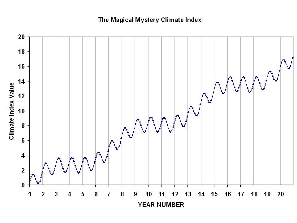
Several commenters were actually very close in their explanation…but Luis Salas gave the actual equation to explain the above plot (and it looks like an “honorable mention” for CatJ). It’s the sum of 3 terms: a linear trend, an annual cycle, and a 6.5 year cycle:
magical-mystery-climate-index-components

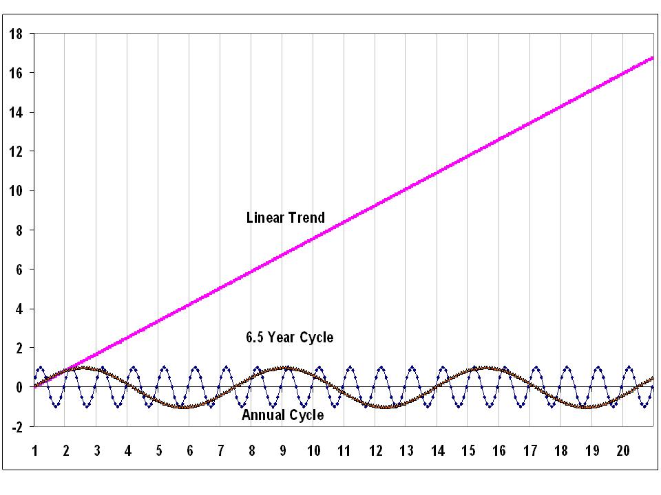
Why did I do this? As a couple of people already guessed, it was mostly to show how a linear trend superimposed upon a cycle can yield periods of rapid change, followed by no change, then rapid change once again. In other words, a linear trend combined with a sinusoidal cycle can lead to plateaus.

Is that what is going on in today’s globally averaged temperature? A warming trend with a natural cycle producing our current warming plateau? I don’t know…but I don’t think we can rule it out. If that is what’s happening, then when warming returns it should be about as strong as before. But….

…but a couple people also alluded to another possibility: that what I have shown as a linear trend is (in nature today) just part of lower frequency oscillation…say the ~60 year cycle in ENSO strength, related to the Pacific Decadal Oscillation (PDO). In that case, it would be possible for there to be a long period of downward trend in temperatures in our future.

I’m really not advocating what the forcing mechanisms are: solar, internal variability, etc. I’m just trying to get people to think in terms of these superimposed signals. (Which, of course, are just mathematical simplifications of what could be the net effect of very complex physical processes).

Only time will tell which is closer to the truth, or whether the real situation might be even more complicated that the possibilities listed above…which would not surprise me at all.


44 Responses to “The Magical Mystery Climate Index: Luis Salas nails it.”

Toggle Trackbacks

  1. Fulco says:

    Roy,

    You are not able to detect trends that have a longer period than say 40 or more units this way. so what will happen at this timescale or larger is unknown.
    But this is a way to deduce a temperature prediction based on PDO and AMO which wil tell you we are going to experience a colder period for more than five decades.
    By the way, Where is your polynomial regression in the temperature charts.

  2. don penman says:

    I think that the trend could also be derived from the up and down components of the oscillations changing relative to each other over time.Seasonal variation would lead to long term variation.

  3. Fonzie says:

    This is why I always disdained the Lindzen argument in “the great global warming swindle” that says that before WW2 when emissions were low (great depression) we had warming but after WW2 with higher emissions (post war boom) there was cooling. AGW theory only means that natural variability will be influenced in an upward (warming that is) direction. Peaks will be higher and troughs won’t be quite as low. Not that this has necessarily happened… A very interesting comment was posted back in october about the callender adjustments to the hadley data set that supposedly created an artificial warming trend. If any one would like to see the “unadjusted” data set you can find the link in the october 2013 archives (located to the right); the blog post is entitled “the social benefit of carbon” dated october 18 and the comment is by “wayne” october 20 6:42pm. He does a nice job of explaining the whole thing, the link is given in the comment.The raw data shows no linear warming trend during the latter part of the twentieth century; that is from 1940 onward…

  4. It is now quite apparent that the main decadal and millennial climate trends can be explained by the 60 year and 1000 year solar cycles. These have been discussed and documented in in a series of posts on my blog at
    http://climatesense-norpag.blogspot.com
    Here is a summary of the conclusions in the last post at that site which was also a guest post on WUWT on Oct 29th
    http://wattsupwiththat.com/2013/10/29/commonsense-climate-science-and-forecasting-after-ar5/
    “In earlier posts on this site http://climatesense-norpag.blogspot.com at 4/02/13 and 1/22/13 I have combined the PDO, Millennial cycle, and neutron trends to estimate the timing and extent of the coming cooling in both the Northern Hemisphere and Globally.

    Here are the conclusions of those posts.

    1/22/13 (NH)

    1) The millennial peak is sharp – perhaps 18 years +/-. We have now had 16 years since 1997 with no net warming – and so might expect a sharp drop in a year or two – 2014/16 -with a net cooling by 2035 of about 0.35.Within that time frame however there could well be some exceptional years with NH temperatures +/- 0.25 degrees colder than that.
    2) The cooling gradient might be fairly steep down to the Oort minimum equivalent which would occur about 2100. (about 1100 on Fig 5) ( Fig 3 here) with a total cooling in 2100 from the present estimated at about 1.2 +/-
    3) From 2100 on through the Wolf and Sporer minima equivalents with intervening highs to the Maunder Minimum equivalent which could occur from about 2600 – 2700 a further net cooling of about 0.7 degrees could occur for a total drop of 1.9 +/- degrees
    4)The time frame for the significant cooling in 2014 – 16 is strengthened by recent developments already seen in solar activity. With a time lag of about 12 years between the solar driver proxy and climate we should see the effects of the sharp drop in the Ap Index which took place in 2004/5 in 2016-17.

    4/02/13 ( Global)

    1 Significant temperature drop at about 2016-17
    2 Possible unusual cold snap 2021-22
    3 Built in cooling trend until at least 2024
    4 Temperature Hadsst3 moving average anomaly 2035 – 0.15
    5 Temperature Hadsst3 moving average anomaly 2100 – 0.5
    6 General Conclusion – by 2100 all the 20th century temperature rise will have been reversed,
    7 By 2650 earth could possibly be back to the depths of the little ice age.
    8 The effect of increasing CO2 emissions will be minor but beneficial – they may slightly ameliorate the forecast cooling and help maintain crop yields .
    9 Warning !! There are some signs in the Livingston and Penn Solar data that a sudden drop to the Maunder Minimum Little Ice Age temperatures could be imminent – with a much more rapid and economically disruptive cooling than that forecast above which may turn out to be a best case scenario.

    How confident should one be in these above predictions? The pattern method doesn’t lend itself easily to statistical measures. However statistical calculations only provide an apparent rigor for the uninitiated and in relation to the IPCC climate models are entirely misleading because they make no allowance for the structural uncertainties in the model set up.

    This is where scientific judgment comes in – some people are better at pattern recognition and meaningful correlation than others. A past record of successful forecasting such as indicated above is a useful but not infallible measure. In this case I am reasonably sure – say 65/35 for about 20 years ahead. Beyond that certainty drops rapidly. I am sure, however, that it will prove closer to reality than anything put out by the IPCC, Met Office or the NASA group. In any case this is a Bayesian type forecast- in that it can easily be amended on an ongoing basis as the Temperature and Solar data accumulate. If there is not a 0.15 – 0.20. drop in Global SSTs by 2018 -20 I would need to re-evaluate.”

    • Fonzie says:

      With the sun being as lazy as it has this could be the acid test. Time will shortly tell if the ” it’s the sun stupid!” crowd is right after all. These are exciting (but hopefully not too chilly) times…

  5. Marvin Gardens says:

    Just saw this and I thought of Dr. Spencer. One of the theme’s of this site is that natural climate variation is important, and it is often asserted that nobody (or nearly nobody) in the climate science ball-game is studying the possibility that natural variation is the cause of observed warming.

    This is from a call for proposals from the NSF. Under the list of “primary topics of focus”

    “Analysis that enhances understanding and predictability of modes of Natural Climate Variability (ranging from intraseasonal to multi- decadal): Activities that focus on the identification, evaluation, and understanding of these modes, (e.g., MJO, ENSO, PDO, and AMO, as well as interactions among these modes) and how these may change in a changing climate, as evidenced in coupled model simulations, are encouraged.”

    http://science.energy.gov/~/media/grants/pdf/foas/2014/SC_FOA_0001036.pdf

  6. Engineer Bob says:

    I like this method of simple curve fitting to the empirical data. Several people have published variations of this. For example, Loehle, C. and N. Scafetta. 2011. Climate Change Attribution Using Empirical Decomposition of Historical Time Series. Open Atmospheric Science Journal 5:74-86.

    The Loehle and Scafetta paper is discussed in
    http://wattsupwiththat.com/2011/07/25/loehle-and-scafetta-calculate-0-66%C2%B0ccentury-for-agw/

  7. KevinK says:

    Dr. Spencer, with respect;

    A very nice demonstration.

    A couple of observations;

    1) If you start with only the data (no a-priori knowledge of the input “forcings”) this is just one set of functions that will produce this output.

    2) This particular set of input functions is not the only unique solution that will produce this result.

    3) For example, there could be (just a hypothetical here) a strong upward linear trend and a weaker downward linear trend that combine to produce the mild upward trend you created.

    4) Without knowledge of all these trends it is not possible to ascertain all of the causes of the final observed result.
    5) Depending on the sampling time and extent it is possible to “mimic” or “approach” a linear trend from a long duration sine wave.

    6) When viewing near the peak of a sine wave lasting thousands of years the observations can look very much like a linear trend.

    7) Near the peak of a sine wave the slope approaches zero, and in fact is zero at the peak and then becomes negative.

    8) The derivative of a sine wave is of course a cosine wave and near the zero crossing this derivative (the slope) looks very much like a linear trend (i.e. the slope is very close to a fixed value for “long” periods of time).

    9) The resolution of the observing instrument will produce an interval on both sides of the peak of a sine wave where it is impossible to accurately determine that the trend is other than what looks like a purely linear trend.

    10) When designing a control system engineers try to avoid operating around a local maxima (or minima) of an observing instrument when possible because noise and resolution limits become problematic. Of course a local maxim can be useful to find a “home” or initial position. But if you want good control of a system you want your observations to have the maximum slope or gain possible.

    In summary, given the total duration of time that the Earth has had a climate a few thousand years of data is pretty sparse when trying to definitively describe all of the trends and cycles producing the observed results.

    Cheers, Kevin.

  8. For fun I created an “good” match to hadcrut3 data using only a sum of sinusoids – no trend and also a sum of sinusoids + polynomial trend.

    The sinusoid only plot doesn’t math early data well, and diverges significantly in future years from the poly plot. The matching is mainly due to a 315 year and 60 year cycle

    The poly trend shows better matching over the hadcrut data to 2013. The matching is mainly the 60 year cycle and polynomial trend.

    The poly trend plot shows that temperatures can be forced into a flat trend until 2020 by a 60 year cycle shown in the plots.
    This is the real significance of these 2 plots. They show how a strong 60y cycle can flatten out the trend for 20 years. But in the background the trend is continuously rising. On the upswing of the 60y cycle the rate of change of temperature increases significantly.

    It should be noted that there is no science in this it is simply curve fitting!!! Consequently it probably has no predictive ability.

    The series of posts are here:
    http://climateandstuff.blogspot.co.uk/search/label/temperature%20synthesis

  9. Antonio (AKA "Un físico") says:

    At present, climate models have nothing to do with cyclical vs. linear management. But on how to keep a lie alive.
    In my view, in late 80′s (cold war was ending) and UN had to struggle for survival. So they started to think in global policies, but the sad fact is that they invented a fictitious science,
    https://docs.google.com/file/d/0B4r_7eooq1u2VHpYemRBV3FQRjA
    in order to provide some kind of reliability for those policies.
    I understand that you might think that my view is another paranoic conspirancy theory from a mad man in the internet. But all this political invasion of science, is explained and justified in Al Gore’s 90′s book “Earth in the Balance: Forging a New Common Purpose”.
    I think that Dr. Spencer’s point: “only time will tell which is closer to the truth”, is not appropriate. I believe that scientist must identify the fallacies in IPCC’s climatic report (as I did) and to make them public. This is the only way for climatic science to keep staying reliable.

    • Fonzie says:

      I would agree that “only time will tell” ain’t the way to go. As the good doctor has oft said you can flip a coin as to whether wel’ll have future warming or not. AND one way or another, they will claim any warming as being anthropogenic. We can’t leave our future up to the toss of a coin…

  10. Dr. Strangelove says:

    The real situation is long-term cooling since 3,300 years ago with four distinct warming periods: Minoan, Roman, Medieval and recent (19 & 20th centuries)

    The warming periods are successively cooler than the previous one. This is based on temperature reconstruction from Greenland GISP2 ice core (Alley; Easterbrook)

    Geologists refer to ca. 8,000 years ago as the interglacial optimum. The world has been cooling since then. The last interglacial lasted 17,000 years. The current one started 18,000 years ago. We may be nearing its end. The ice age is coming. Or to be precise, we are still in an ice age.

    • Fonzie says:

      Yeah, let’s hope that al gore and friends (Al et al) are right !!!

    • JohnKl says:

      Dr. Strangelove,

      Louis Agassiz convinced Charles Lyell that a prior ICE AGE existed based on the evidence of moraines, earth fissures and other geological disturbances found in western Europe. From what I’ve learned, the massive water and/or ice required to generate them has no known cause in the last 5+k years of recorded profane history. Permafrost blankets regions once supporting large animals and tropical vegetation during this period. A prior colder and wetter period likely existed. Your last point “we are still in an ice age” I believe will prove the more accurate description.

      Have a great day!

      • Dr. Strangelove says:

        The present ice age is called Quaternary glaciation. Common knowledge to geologists but an inconvenient truth the warmists conveniently forget. The present ice age is obvious. The polar sea ice is larger than Europe and US combined. The ice sheet in Antarctica alone is enough to bury all the land in the world under 660 feet of ice. If the world were not in an ice age, the polar region would be ice free.

        And the long-term cooling trend will continue according to a seminal paper by John Imbrie, a pioneer in the study of ice ages.

        “Ignoring anthropogenic and other possible sources of variation acting at frequencies higher than one cycle
        per 19,000 years, this model predicts that the long-term cooling trend which began some 6000 years ago will continue for the next 23,000 years.”

        http://www.whoi.edu/cms/files/imbrie80sci_53864.pdf

  11. RichardLH says:

    Ah well. My mistake in choosing a third term of 7 years left me with residuals that needed explaining. My bad.

    Perhaps you can ask the ‘winners’ to explain their methodology as that may prove interesting.

    As to ‘real world’ climate values. There are some problems with such simple explanations.

    Linear trends are almost always a form of self deception. Either you are proposing but not stating some form of ‘hockey stick’ with a flat set of values at some point in the past to conform to know historical values or the rising (for upwards trends) edge of a cyclic form with a unstated period, magnitude and phase.

    As the 60 year cycle shows up in lots of temperature and related records to not assign a value, range and phase to that ignores all that evidence completely.

    An even simpler problem is that of ‘leap years’. We all know that a true solar year is 1461 days (4 years) and that the temperature response of land and ocean is significantly different but we still use 365 (and forget the remainder) day normals to analyse temperature records.

    • Luis Salas López says:

      Hello RichardLH:

      Surely the ideal is to perform Fourier analysis, but I do not know.

      My method was:
      1 – I wrote a first test formula.
      2 – Then I calculated the difference between the data of Roy W. Spencer and calculated that my formula.
      3 – In another cell I calculated the sum of these differences.
      4 – I was adjusting parameters using the “Solver” Add-in of Excel.
      5 – I removed or added parameters and returning to step 2, until the difference between the data of Roy W. Spencer and calculated that my formula was zero.

      The method is trial and error. It is unorthodox. So I think a Fourier analysis would have been right.

      Thanks to Roy W. Spencer, for the challenge and the award. 🙂

    • Cat J says:

      If anyone still cares . . .

      I eyeballed the linear trend and guessed it was 16 (nice round number, right?), then took the FFT of the data with the linear trend removed. This clearly showed two frequencies. So I dashed off a hasty guess early in the day.

      Later I was procrastinating at work so I looked again. The problem with the FFT is that the data is not truly periodic on the observation window. It was clear what the high-frequency component was, so I wrote a little Matlab script to plot the error for a range of second frequencies around the one given by the FFT. The error is linear when you get the second frequency nailed down, and that gives you the trend and offset.

      Not very elegant, I admit. But effective.

      BTW, it would have been much harder to get the exact formula if Roy had not chosen round numbers for the two frequencies and amplitudes. Or made the frequencies themselves vary in time.

      Cat

  12. lemiere jacques says:

    what????no trick at all ?? i had to remember all trigonometry formula ( for a few minutes) to figure out what was the trick.

    quite a weird thing…so obvious…

    on a mathematical point of view , the re probably other solutions, because of the narrow domain of your graphically defined function.

    the only way to graph a sinuid function right is to plot it on a given number of period and give the way to plot it every else were.

    In fact, whay if your function looks like a sin one on a few periods and is flat else where like a wavelet…

    well sorry…just want a say..what no trick????
    an on a mathematicla point of view your function fit the curve displaid on the interval..that s all..and it is VERY different from the fact the function is the one and only that does.
    And overall you MUST give the way to plot it elsewhere. then an anly then ther will be very little room for another “solution”.

    but no harm it was nice tio try to remember formula

  13. joe bastardi says:

    Roy
    Gray has talked about this since the 1970s I am a big sun/ocean/stochastic event supporter. The Paper by Bill Gray is not gospel, but could perhaps be on of the books of the climate bible

    http://typhoon.atmos.colostate.edu/Includes/Documents/Publications/gray2012.pdf

    • Dr. Strangelove says:

      Joe
      I believe it is not coincidence that THC has a cycle of about 1,000 years and the warm periods (Minoan, Roman, Medieval and present) have an interval of about 1,000 years.

    • lgl says:

      “could perhaps be on(e) of the books of the climate bible”

      With all the flaws already in fig.1 and 2, don’t think so.

  14. Joe Bastardi Compare Gray’s approach with that outlined at 25/6:57pm above Also at
    http://climatsense-norpag.blogspot.com
    looks like we are all on the same page.
    Just need to get the message through to the MSM and Obama administration!!

  15. alex says:

    Then there are Milankovitch Cycles of course, cycles that trump the higher frequency once every 400K, 100K years, 12K years + some more

    http://www.eoearth.org/view/article/154612/

    • Chic Bowdrie says:

      alex,

      Would it be better to say the shorter cycles obscure our contemporary view of the longer cycles rather than be trumped by them? Cycles longer than a 1000 years with an amplitude of at least a degree or two will look like linear trends in the short term. Maybe Luis or others can come up with a hypothetical equation going back 2000 years to illustrate.

  16. alex says:

    errata corrige:
    ///higher frequency ones//

  17. lemiere jacques says:

    the point is you can see almost what you want to see…and don’t forget errors bar in the date, don’t forget the data is not homogeneous at all ( “corrections”)…

    the only thing that helps a bit to see if what you think was right is your ability to predict…

    if you had the components right, ie understanding of the physics, then your prediction will be right ..if not… either you re wrong or the physics have changed.

    • Chic Bowdrie says:

      Yes, I agree we see what we want to see. This is a microcosm of the whole global warming issue. People saw the temperature-CO2 correlation of the last century and jumped to the AGW conclusion.

      I suspect that Dr. Spencer has purposefully designed this blog post to illustrate his oft mentioned plea to give natural factors at least an equal billing in climate models instead of starting with CO2 as the primary component.

  18. Christopher Game says:

    It seems that we are using the term ‘forcing’ for two things, external and internal time-dependent quantities that appear on the right hand side of an ordinary differential equation for the time derivative of a variable that is determined by the dynamics of our system. An external driver is in this IPCC language called a forcing, even when, like CO2, it is more conventionally called a time-dependent parameter of the system. But quantities that are functions of dependent state variables of our system and appear as additive terms on the right hand side of our differential equation also now seem to be called forcings.

  19. B Parsons says:

    When are you going to skip the freshman calculus and give us your comments on recent literature such as ozone ban may have slowed growth, or recent modelling that shows the El Nino dominates the slow in warming, or recent work on arctic algae that shows the last 150 years have unusual reduction of ice cover. For a hard working scientist you are very careful to ignore anything in the recent literature that might actually shed some real light on all this instead of fooling around with this trivial stuff, that we all learned when we were t4eeenagers? I don’t think that you are objective, well read or very hard working.

  20. Trends do not forecast future climate changes.

    What this climate index assumes is the same circumstances that produced the linear climate trend ,the 6.5 year cycle ,and annual cycle are going to continue as is going forward and thus some kinds of conclusions can be drawn from this, for the future climate.

    Will not work and if this same climate index was used at various times in the past just prior to an abrupt climate change that was about to take place this index would have been oblivious to that pending abrupt climate change.

  21. I am quite confident that if prolonged quiet solar conditions continue going forward that the global temperature trends will be down. In fact I expect to see this trend in global temperatures to set in within 6 months of the ending of the maximum of solar cycle 24, which is not that far off.

  22. SOLAR CLIMATE MECHANISMS AND CLIMATE PREDICTION

    MECHANISM ONE

    One solar climate mechanism/connection theory which has much merit in my opinion, is as follows:

    A BRIEF OVERVIEW. At times of low solar irradiance the amounts of sea ice in the Nordic Sea increase, this ice is then driven south due to the atmospheric circulation (also due to weak solar conditions) creating a more northerly air flow in this area.(-NAO) This sea ice then melts in the Sub Polar Atlantic,releasing fresh water into the sub- polar Atlantic waters, which in turn impedes the formation of NADW, which slows down the thermohaline circulation causing warm air not to be brought up from the lower latitudes as far north as previous while in lessening amounts.

    This perhaps can be one of the contributing solar/climate connection factors which brought about previous abrupt N.H. cool downs during the past.

    This makes much sense to me.

    NAO= NORTH ATLANTIC OSCILLATION
    NADW= NORTH ATLANTIC DEEP WATER

    To elaborate on the above, when the sun enters a prolonged solar minimum condition an overall reduction takes place in solar spectral irradiance, namely in UV light (wavelengths less then 400 nm). The shorter the wavelength,the MUCH greater the reduction.

    UV light reduction likely will cause ocean heat content and ocean surface temperatures to drop, due to the fact that UV light in the range of 280 nm-400nm penetrates the ocean surface to depths of 50-100 meters. A reduction in UV (ultra violet) light then should have a profound effect on the amount of energy entering the ocean surface waters from the sun extending down to 50-100 meters in depth, resulting in cooler ocean temperatures.

    This ties into what was said in the above in that if ocean waters in high latitudes such as the Nordic Sea, were to be subject to cooling the result would be much more sea ice which could impede the strength of the thermohaline circulation promoting substantial N.H. cooling.

    Adding to this theory is fairly strong evidence that a decrease in UV light will result in a more meridional atmospheric circulation (which should cause more clouds, precipitation and snow cover for the N.H.), due to changes in ozone distribution in a vertical/horizontal sense which would cause the temperature contrast between the polar areas of the stratosphere and lower latitude areas of the stratosphere to lesson, during prolonged solar minimum periods. Ultra Violet light being likely the most significant solar factor affecting ozone concentrations ,although not the only solar factor.

    This could then set up a more -NAO, (high pressure over Greenland) which would promote a more Northerly flow of air over the Nordic Sea, bringing the sea ice there further South.

    MECHANISM TWO

    A reduction of the solar wind during a prolonged solar minimum event would cause more galactic cosmic rays to enter the earth’s atmosphere which would promote more aerosol formation thus more cloud nucleation. The result more clouds higher albedo, cooler temperatures.

    Compounding this would be a weaker geo magnetic field which would allow more galactic cosmic ray penetration into the atmosphere , while perhaps causing excursions of the geo magnetic poles to occur in that they would be in more southern latitudes concentrating incoming galactic cosmic rays in these southern latitudes where more moisture would be available for the cosmic rays to work with, making for greater efficiency in the creation of clouds.

    MECHANISM THREE

    MILANKOVITCH CYCLES overall favor N.H. cooling and an increase in snow cover over N.H high latitudes during the N.H summers due to the fact that perihelion occurs during the N.H. winter (highly favorable for increase summer snow cover), obliquity is 23.44 degrees which is at least neutral for an increase summer N.H. snow cover, while eccentricity of the earth’s orbit is currently at 0.0167 which is still elliptical enough to favor reduced summertime solar insolation in the N.H. and thus promote more snow cover.

    In addition the present geographical arrangements of the oceans versus continents is very favorable for glaciation.

    MECHANISM FOUR

    High latitude major volcanic eruptions correlate to prolonged solar minimum periods which translates to stratospheric warming due to an increase in SO2 particles while promoting more lower troposphere cooling.

    One theory of many behind the solar/volcanic connection is that MUONS, a by product of galactic cosmic rays can affect the calderas of certain volcanoes by changing the chemical composition of the matter within the silica rich magma creating aerosols which increase pressure in the magma chamber and hence lead to an explosive eruption.

    Muon densities increase more in higher latitudes at times of weak solar magnetic activity, which is why volcanic activity in the higher latitudes will be affected more by this process.

    These four mechanisms make a strong case for a solar /climate connection in my opinion, and if the prolonged solar minimum meets the criteria I have mentioned going forward and the duration is long enough I expect global cooling to be quite substantial going forward.

    THE CRITERIA

    Solar Flux avg. sub 90

    Solar Wind avg. sub 350 km/sec

    AP index avg. sub 5.0

    Cosmic ray counts north of 6500 counts per minute

    Total Solar Irradiance off .015% or more

    EUV light average 0-105 nm sub 100 units (or off 100% or more) and longer UV light emissions around 300 nm off by several percent.

    IMF around 4.0 nt or lower.

    The above solar parameter averages following several years of sub solar activity in general which commenced in year 2005..

    IF, these average solar parameters are the rule going forward for the remainder of this decade expect global average temperatures to fall by -.5C, with the largest global temperature declines occurring over the high latitudes of N.H. land areas.

    The decline in temperatures should begin to take place within six months after the ending of the maximum of solar cycle 24.

    NOTE 1- What mainstream science is missing in my opinion is two fold, in that solar variability is greater than thought, and that the climate system of the earth is more sensitive to that solar variability.

    NOTE 2- LATEST RESEARCH SUGGEST THE FOLLOWING:

    A. Ozone concentrations in the lower and middle stratosphere are in phase with the solar cycle, while in anti phase with the solar cycle in the upper stratosphere.

    B. Certain bands of UV light are more important to ozone production then others.

    C. UV light bands are in phase with the solar cycle with much more variability, in contrast to visible light and near infrared (NIR) bands which are in anti phase with the solar cycle with much LESS variability.

    This is my latest take, time will tell.

  23. Separating periods of time or frequencies in a global temperature spectrum is the first step to find any coherence to functions in nature. But first it is necessary to remove the volcano drops from the spectrum. The global temperature spectrum can be analysed for time periods of millennia to month. Some time periods are locked to the Earth axis wobble spectrum which is in coherence to the ENSO spectrum, http://www.volker-doormann.org/images/ensoshift1.gif
    some periods can related to solar tide functions. http://www.volker-doormann.org/images/minus1960.gif , http://www.volker-doormann.org/images/hegerl_900.gif . It seems, it is not a good way to start with sine functions without any geometry in nature, if the natural functions have other forms, or are itself a resonance spectrum of integer modes, like the ENSO spectrum; but it is a good way in general to analyse the temperature spectra and find coherence to real nature.

    V.

  24. Temperature ALWAYS is in phase with the inverse of Ice Extent and Albedo.

    It snows more when oceans are warm and polar sea ice is thawed.

    It snows less when oceans are cold and polar sea water is frozen.

    The Polar Sea Ice Cycles matured as the Earth temperatures became more tightly bounded.

    Look at the data.

  25. Jama Stimac says:

    hehe bookmaked. Keeping this for future reference appreciated heaps bro.

  26. aaron says:

    A solar forcing likely acts primarily on the oceans and dark, moist surfaces (though mostly over the oceans as land produces aerosols, so variation in cloud formation is only likely to happen far away from land).

    Say you have a 11yr effect, but the heat goes into the ocean based on above, which has a much more inert temperature and is very chaotic and cyclical. You wouldn’t see much of an 11 year cycle, but effects over the phases of the ocean cycles.

    Also consider the possibilty that the hemi-sphere of solar activity and polarity make a difference the strength of the solar effect (say there is a slight directionality to the particular cosmic rays that affect cloud nucleation ions). There may be a 22yr signal, rather than 11.

    Now, knowing that we can’t observe low cloud cover well, perhaps we can see a signal by looking more specifically where we would expect an effect. The effect is only likely to be observable where there are few similar cloud nucleation particles. Can’t someone make a for areas with high concentrations these land based particles?

    Now consider again that we can’t observe low cloud cover well. Can we instead observe the rate of formation. Is there a specific set of wavelenths that is emitted when water vapor condense at low altitudes and can this be observed?

    • aaron says:

      “Can’t someone make a for areas with high concentrations these land based particles?”

      The question should be, “Can’t someone make a MASK for areas with high concentrations these land based particles?”

  27. I read this piece of writing completely concerning the comparison of most recent and preceding technologies, its awesome article.

  28. I truly enjoy looking at on this internet site, it contains good articles.

Leave a Reply