Australia Surface Temperatures Compared to UAH Satellite Data Over the Last 40 Years

April 3rd, 2019 by Roy W. Spencer, Ph. D.

Summary: The monthly anomalies in Australia-average surface versus satellite deep-layer lower-tropospheric temperatures correlate at 0.70 (with a 0.57 deg. C standard deviation of their difference), increasing to 0.80 correlation (with a 0.48 deg. C standard deviation of their difference) after accounting for precipitation effects on the relationship. The 40-year trends (1979-2019) are similar for the raw anomalies (+0.21 C/decade for Tsfc, +0.18 deg. C for satellite), but if the satellite and rainfall data are used to estimate Tsfc through a regression relationship, the adjusted satellite data then has a reduced trend of +0.15 C/decade. Thus, those who compare the UAH monthly anomalies to the BOM surface temperature anomalies should expect routine disagreements of 0.5 deg. C or more, due to the inherently different nature of surface versus tropospheric temperature measurements.

I often receive questions from Australians about the UAH LT (lower troposphere) temperature anomalies over Australia, as they sometimes differ substantially from the surface temperature data compiled by BOM. As a result, I decided to do a quantitative comparison.

While we expect that the tropospheric and surface temperature variations should be somewhat correlated, there are reasons to expect the correlation to not be high. The surface-troposphere system is not regionally isolated over Australia, as the troposphere can be affected by distant processes. For example, subsidence warming over the continent can be caused by vigorous precipitation systems hundreds or thousands of miles away.

I use our monthly UAH LT anomalies for Australia (available here), and monthly anomalies in average (day+night) surface temperature and rainfall (available from BOM here). All monthly anomalies from BOM have been recomputed to be relative to the 1981-2010 base period to make them comparable to the UAH LT anomalies. The period analyzed here is January 1979 through March 2019.

Results Before Adjustments

A time series comparison between monthly Tsfc and LT anomalies shows warming in both, with a Tsfc warming trend of +0.21 C/decade, and and a satellite LT trend of +0.18 C/decade:

Fig. 1. Australia average surface temperature (red) and satellite lower tropospheric temperature (LT, blue) anomalies from January 1979 through March 2019.

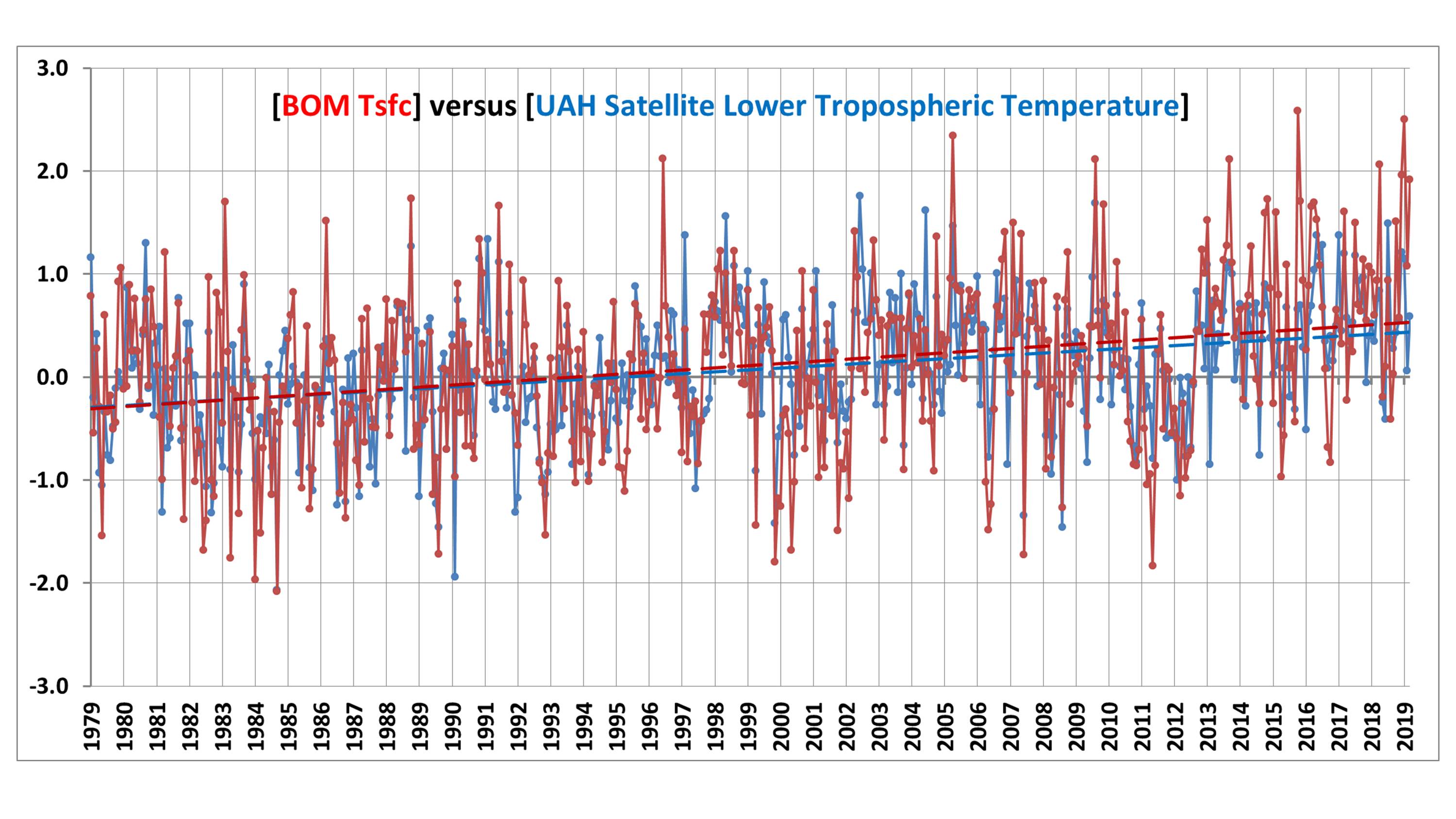
The correlation between the two time series is 0.70, indicating considerable — but not close — agreement between the two measures of temperature. The standard deviation of their difference is 0.57 deg. C, which means that people doing a comparison of UAH and BOM anomalies each month should not be surprised to see 0.6 deg. C differences (or more).

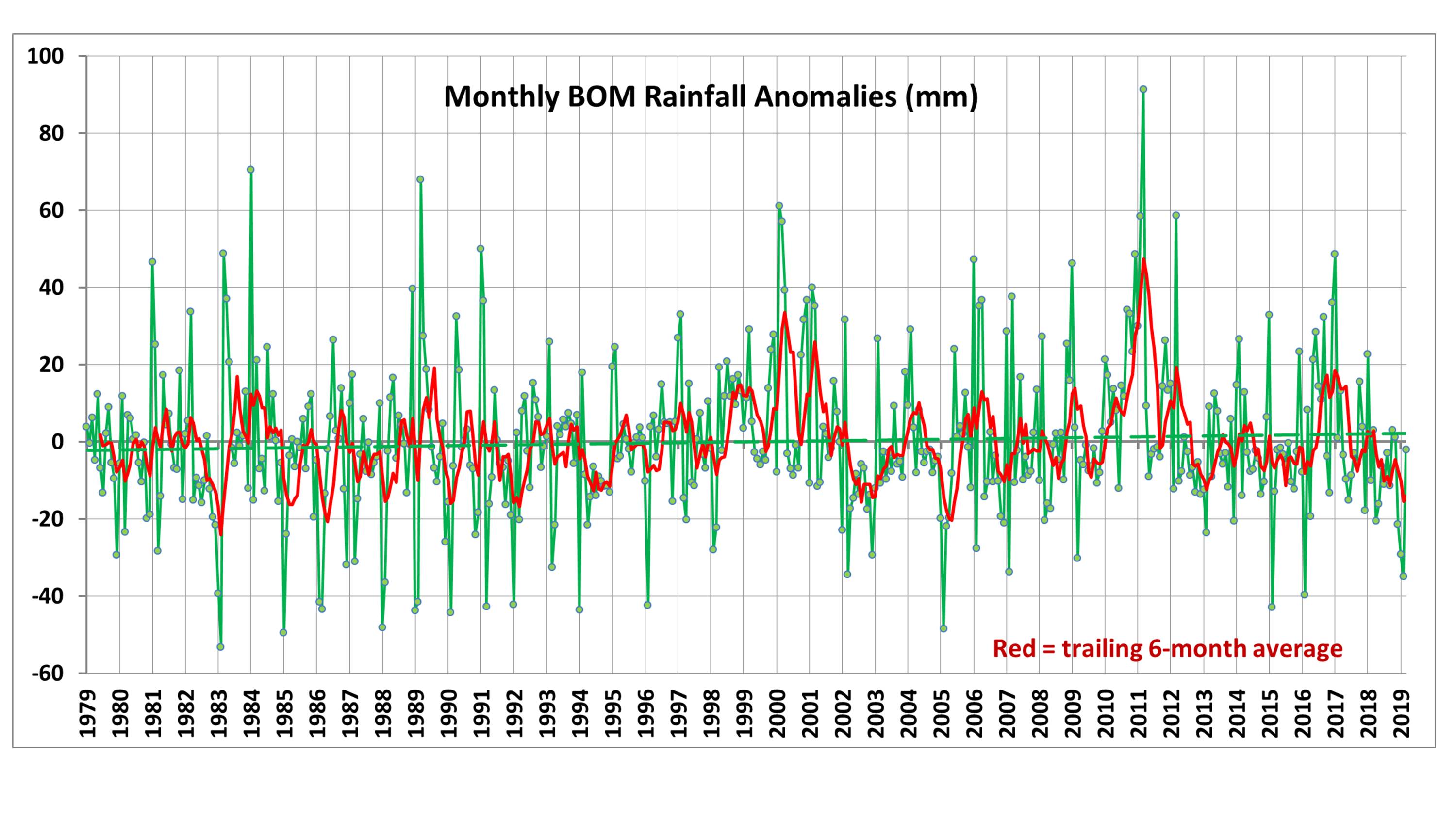
Part of the disagreement comes from rainfall conditions, which can affect the temperature lapse rate in the troposphere. For reference, the following plot shows Australian precipitation anomalies for the same period:

Fig. 2. Australia precipitation anomalies from January 1979 through March 2019.

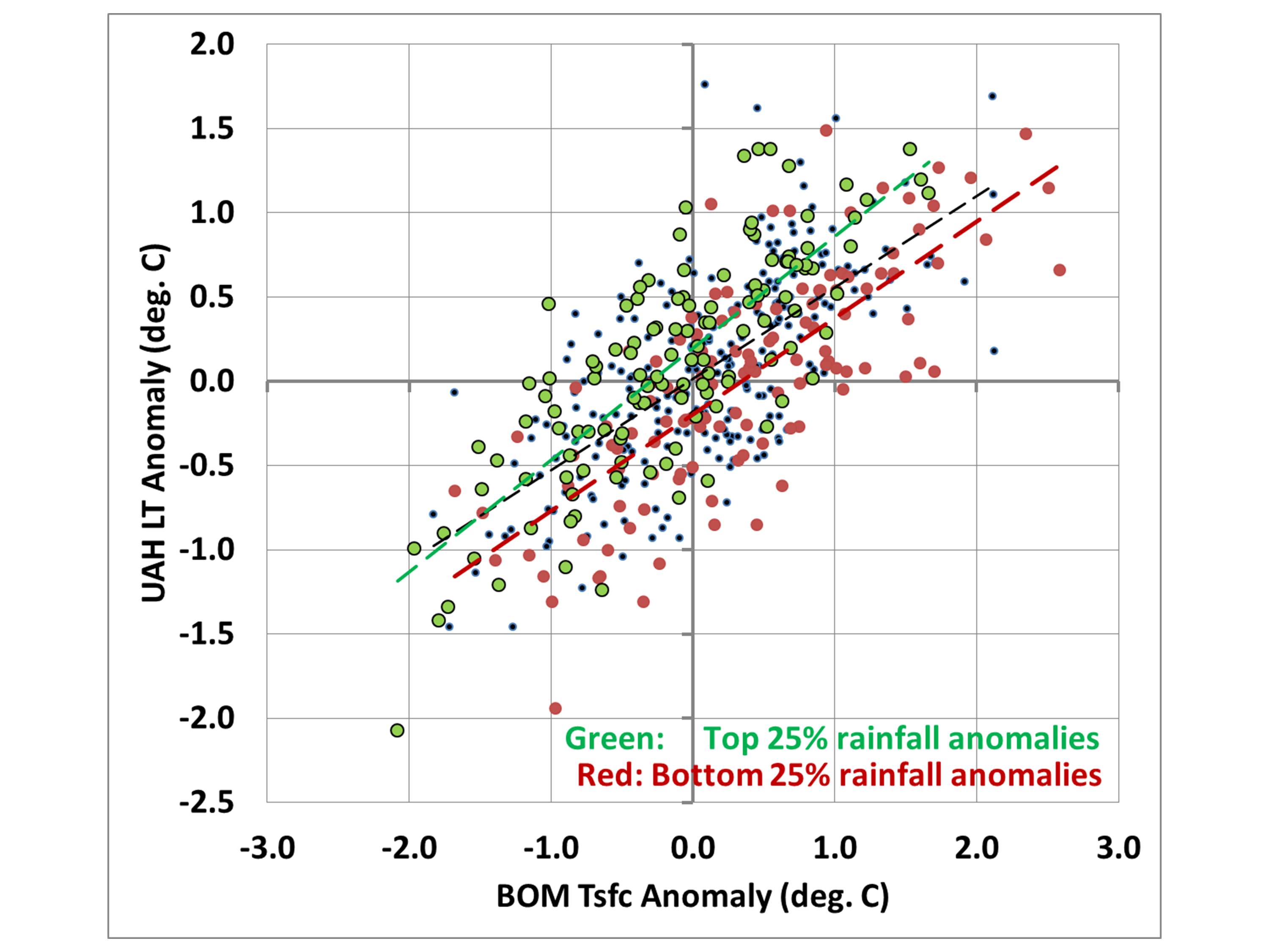
If we take the data in Fig. 1 and create a scatter plot, but show the months with the 25% highest precipitation anomalies in green and the lowest 25% precipitation in red, we see that drought periods tend to have higher surface temperatures compared to tropospheric temperatures, while the wettest periods tend to have lower surface temperatures compared to the troposphere:

Fig. 3. Scatterplot of the data in Fig. 1, but with color coding of those months with the 25% highest (green) and lowest (red) precipitation departures from average.

A More Apples-to-Apples Comparison

Comparing tropospheric and surface temperatures is a little like comparing apples and oranges. But one interesting thing we can do is to regress the surface temperature data against the tropospheric temperatures plus rainfall data to get equations that provide a “best estimate” of the surface temperatures from tropospheric temperatures and rainfall.

I did this for each of the 12 calendar months separately because it turned out that the precipitation relationship evident in Fig. 3 was only a warm season phenomenon. During the winter months of June, July, and August, the relationship to precipitation had the opposite sign, with excessive precipitation being associated with warmer surface temperature versus the troposphere, and drought conditions associated with cooler surface temperatures than the troposphere (on average).

So, using a different regression relationship for each calendar month (each month having either 40 or 41 years represented), I computed a satellite+rainfall estimate of surface temperature. The resulting “satellite” time series then changes somewhat, and the correlation between them increases from 0.70 to 0.80:

Fig. 4. As in Fig. 1, but now the satellite data are used along with precipitation data to provide a regression estimate of surface temperature.

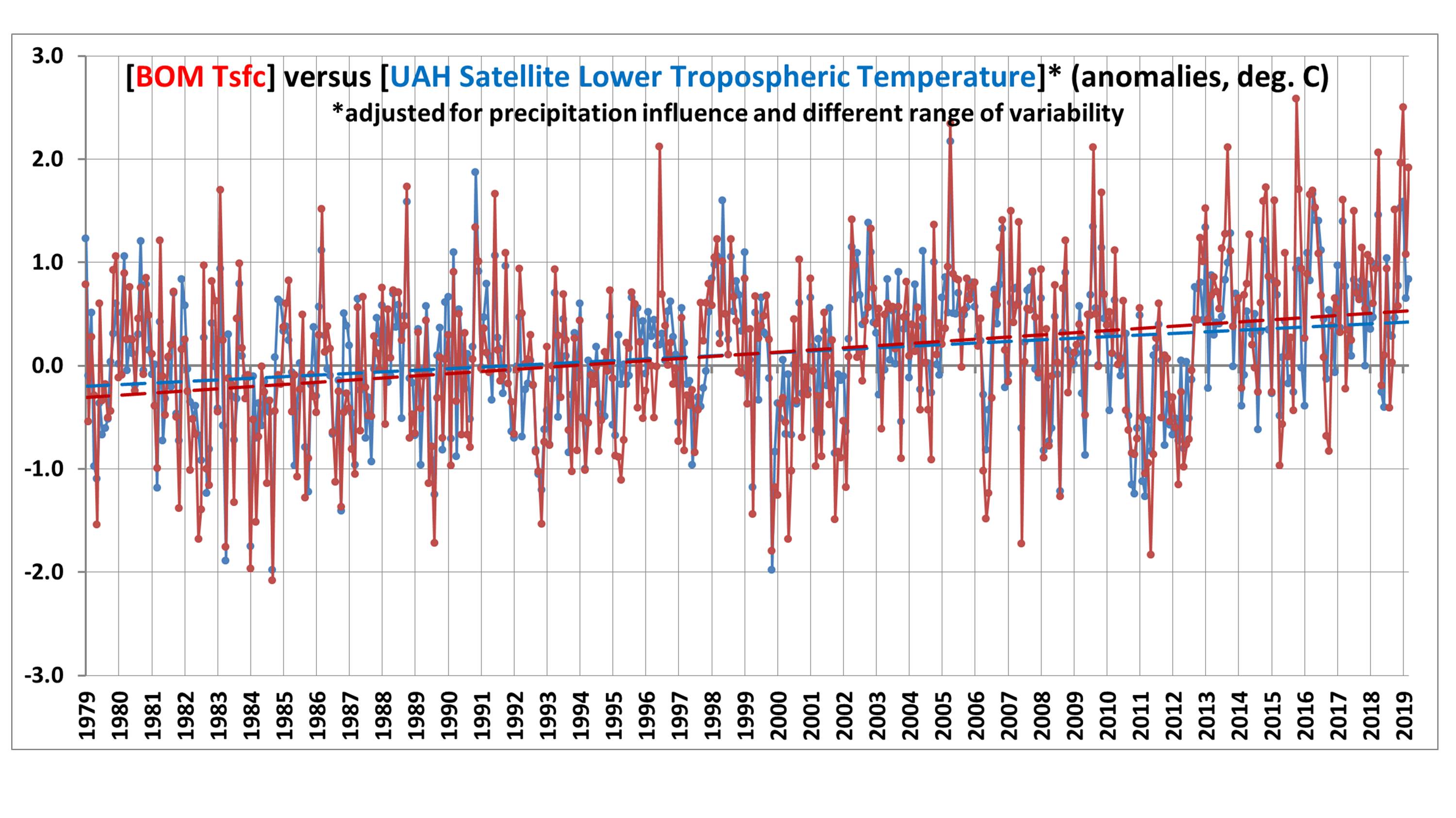
Now the “satellite-based” trend is lowered to +0.15 C/decade, compared to the observed Tsfc trend of +0.21 C/decade. I will leave it to the reader to decide whether this is a significant difference or not.

To make the differences in Fig. 4 a little easier to see, we can plot the difference time series between the two temperature measures:

Fig. 5. Difference between the two time series shown in Fig. 4.

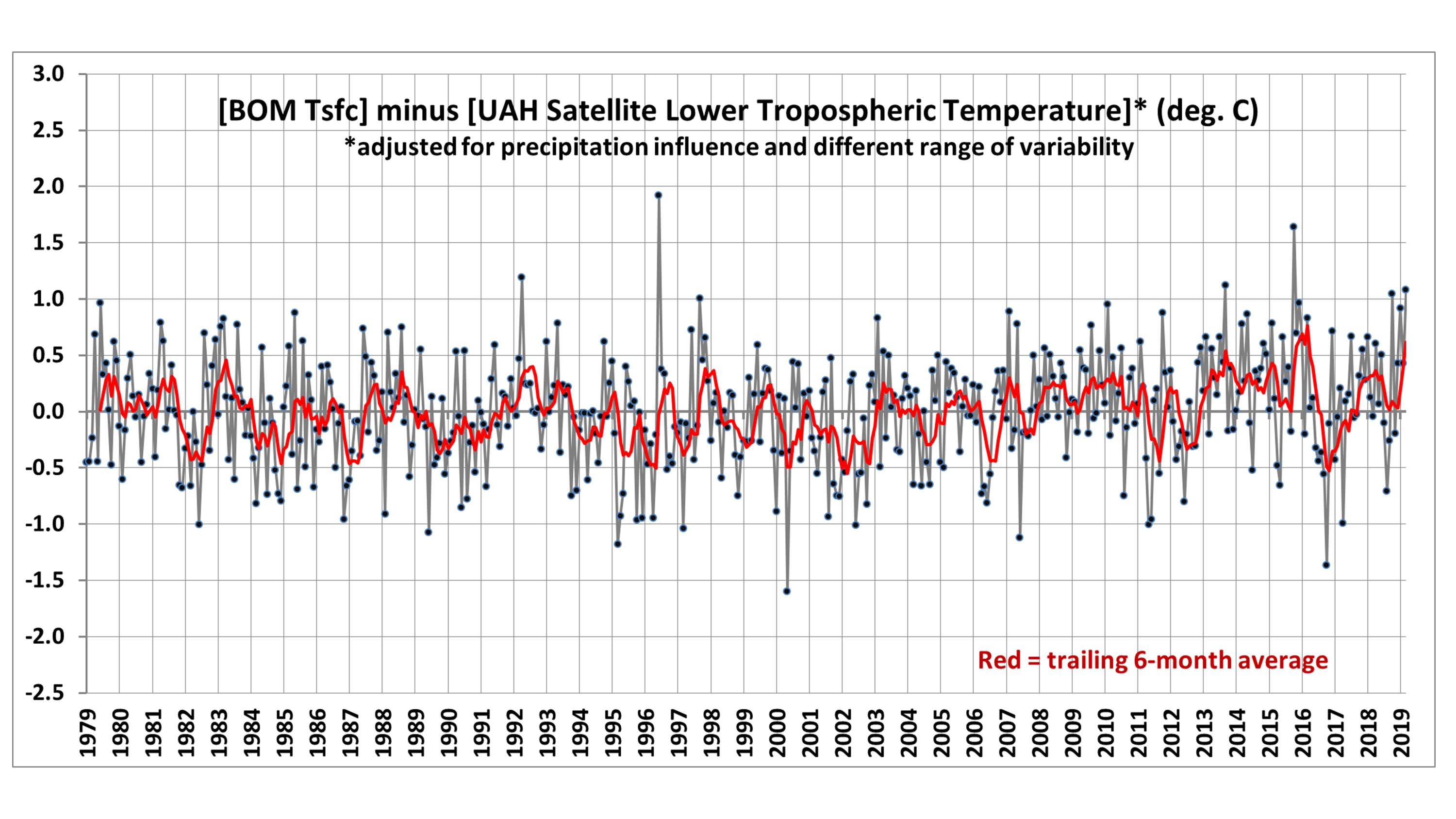
Now we can see evidence of an enhanced warming trend in the Tsfc data versus the satellite over the most recent 20 years, which amounts to 0.40 deg. C during April 1999 – March 2019. I have no opinion on whether this is some natural fluctuation in the relationship between surface and tropospheric temperatures, problems in the surface data, problems in the satellite data, or some combination of all three.

Conclusions

The UAH tropospheric temperatures and BOM surface temperatures in Australia are correlated, with similar variability (0.70 correlation).
Accounting for anomalous rainfall conditions increases the correlation to 0.80. The Tsfc trends have a slightly greater warming trend than the tropospheric temperatures, but the reasons for this are unclear. Users of the UAH data should expect monthly differences between the UAH and BOM data of 0.6 deg. C or so on a rather routine basis (after correcting for their different 30-year baselines used for anomalies: BOM uses 1961-1990 and UAH uses 1981-2010).


57 Responses to “Australia Surface Temperatures Compared to UAH Satellite Data Over the Last 40 Years”

Toggle Trackbacks

  1. barry says:

    Thanks for this.

    To reach out across the water, how does this compare with the other national indices included in UAH data for NOAA: the USA?

  2. MrZ says:

    Hi Roy!

    Thanks for the study.
    This is not April 1st! Here is an example what spread you get depending on how you interpret the surface data.
    http://cfys.nu/videos/Overview.avi
    I am using Sweden in this specific example but the same is true for any region.
    You need to download and select player before you can hear my broken English.

  3. MrZ says:

    Clarification!
    April 1st was related to a joke the other day NOT your study. I am clumsy sometimes…

  4. Stephen P Anderson says:

    Doc,
    It looks like to me it is flat from 1979 to 2012 and then it shifts up 0.6C.

  5. Patrick says:

    0.06 difference over 4 decades = -0.24C difference. That’s only in 1 country. Right? Australia is less than 3 million square miles. How does that reconcile with ocean ARGO data around Australia?

    • goldminor says:

      Here is another thought which always gets left out of the conversation when discussing the SH. Why don’t we see similar heat waves affecting South Africa or South America? Australia has always been known for its high temps ever since it was first colonized.

      Alarmists like to focus on Australia alone as if it was the only land mass in the SH. I suppose that they don’t want to discuss the other land masses as there goes the story that global warming is actually global in its extent.

    • Nate says:

      Hey goldminor!

      Howd that prediction of La Nina go last summer?

      • goldminor says:

        The answer to your question is obvious to both of us. However, just for the record, and for those who may wonder, I did miss that prediction completely.

        What about my comment above though. Let’s see how honest you will be in regards to what I have pointed out that it is only Australia showing high temps, and that Australia has always been known for the same ever since the first colonists arrived there.

        • Bobdesbond says:

          Here in Sydney we have a 160-year temperature record. We are currently on an 87-month run of consecutive above-average monthly average temperatures. You seem to be implying that “hot” is an absolute concept which doesn’t allow for variation.

  6. MikeR says:

    Roy,

    Over at KensKingdom, Ken Stewart has done some really good work on the relationship between rainfall and UAH temperatures for Australia.

    See https://kenskingdom.wordpress.com/2015/11/20/why-are-surface-and-satellite-temperatures-different/ .

    There are also follow ups at

    https://kenskingdom.wordpress.com/2015/11/29/rainfall-and-temperatures-part-2/ and

    https://kenskingdom.wordpress.com/2015/12/02/rain-and-surface-temperature-part-3/

    • Ken Stewart says:

      Thanks Mike R!

      And Dr Spencer, if you look at North Australian rainfall (and in the northern wet season (Nov-April) timeframe), all available from the BOM website, you will find similar or higher correlation with Tmax for all of Australia. Tropical rainfall is massive.

      Ken Stewart

  7. Greg Goodman says:

    Dr Spencer. I would once again draw your attention to the problem of regression dilution when dealing with such noisy scatter plots. Both your OLS slopes are visible too low. This is probably affecting the effectiveness of you attempted corrections.

    I invite you to do the regression with the axes swapped and compare the results. The true best fit probably lies between the two.

    There are various bisectional methods for guessing where between the two results you should take the estimated slope. Geometric mean of the two slopes is one solution. See whether that improved correlation of the adjusted time series.

    More detail here:
    https://climategrog.wordpress.com/2014/03/08/on-inappropriate-use-of-ols/

    best regards. Greg

    [Yes, I am familiar with the issue, and have often mentioned it to others in the context of diagnosing radiative feedbacks from regressions between radiative flux and temperature. In that case, the correlations are low and the regular OLS regression gives a feedback biased low, which then suggests too high of a climate sensitivity. But the problem does not exist when using regression to estimate trends, because there are no errors in one of the variables (time). Otherwise, I agree with you. -Roy]

    • Greg Goodman says:

      here is an example of two slopes using some synthetic data : linear slope + noise.

      https://climategrog.wordpress.com/?attachment_id=853

      The true slope is 3.0, the regression slope comes out a 0.58 ! This is not a pedantic detail.

    • barry says:

      That 0.58 regression slope looks like it has been calculated in a non-normal fashion. An OLS regression would have given a result close to the original. What have you done here to get 0.58?

      Where are your CIs?

    • barry says:

      Ok, the 0.58 is a better fit to the data (I’m a bit colour blind) than the 3.0. The random generator has done something funny here. Those anomalies are a wild departure from a random result.

      I’d suggest running that random generator many times. I suspect you got one of those flukes of statistics, or something wrong with the code.

      What happens if you generate a hundred of these? Does this mismatch appear with any regularity?

      • I’ve done many of these experiments before using random noise added to both variables. You can get a wide variety of results, depending upon how much data you have. But in general I agree the regression slope will be biased low *IF* the correlations are low *AND* there are errors in both variables (which isn’t the case for OLS trends over time, since time has no error).

  8. phi says:

    There is a fairly simple technique for comparing TLTs to surface temperatures. TLT are treated as a simple proxy for surface temperature by calibrating it on the detrended series.

    Using the annual values 1979 to 2017, I get in global (Had_Crut and UAH 6.0):

    – Had_Crut trend: +0.17 ° C per decade,
    – Proxy factor 0.63 (tropospheric amplification: 1.59),
    – TLT proxy trend: +0.09 ° C per decade.
    – Divergence 0.08 ° C per decade.

    With the same technique, I obtain a divergence of 0.15 ° C per decade for the lands of the Northern Hemisphere (tropospheric amplification : 1.00).

    • The trouble is that we really don’t know what “tropospheric amplification” factor should be used… it depends upon water vapor feedback, the free-tropospheric component of which isn’t really known. Without knowing this, we really don’t know whether tropospheric temperature trends are inconsistent with surface temperature trends.

      • phi says:

        Don’t you think that the empirical method is a satisfactory solution?
        That is, estimating tropospheric amplification on the basis of the ratio between standard deviations of detrended TLT and detrended surface temperature.

      • phi says:

        I did a quick check, there is practically no difference in the ratio between 1979 to 1998 and 1999 to 2017 for the detrended series. It seems to me that this means a great stability of amplification and relative humidity.

    • There is the matter that (as I see things) the tropospheric amplification varies with the cause of the temperature change. ENSO events affect satellite-measured lower troposphere and the middle troposphere much more than longer term global temperature changes do, for a given amount of surface temperature change.

      • phi says:

        This is theoretically possible but it is speculative and this would mean that long-term warming is accompanied by a decrease in relative humidity. However, there is no such thing. There is no downward trend in relative humidity. Conclusion: the amplification factor does not seem to vary with the cause.

    • phi says:

      A few words to contextualize these divergence estimates.

      It has been known since 2009 that paleoclimatologists can not properly connect proxies to instrumental temperatures.

      Phil Jones :
      “Ive just completed Mikes Nature trick of adding in the real temps to each series for the last 20 years (i.e., from 1981 onwards) and from 1961 for Keiths to hide the decline.”

      Keith Briffa :
      “We dont have a lot of proxies that come right up to date and those that do (at least a significant number of tree proxies) [show] some unexpected changes in response that do not match the recent warming.”

      The iconic Hide the Decline proxy is the MXD data collected by Schweingruber. It covers the northern hemisphere quite reasonably. This collection can be calibrated using the same technique used here for TLTs. The divergence obtained from 1940 to 1994 is 0.1 C per decade.

      It should now be clear that it is not TLTs, MXDs, TRWs, glaciers, sea levels and so on that each have a different fundamental problem but that the instrumental surface temperatures are seriously biased.

    • phi says:

      Oups, erratum.

      Had_Crut and UAH global 1979 to 2017 :

      – Had_Crut trend 0.15 C per decade
      – TLT trend 0.13 C per decade
      – Proxy factor 0.86 (troposphgeric amplification 1.16)
      – TLT proxy trend 0.11 C per decade
      – Divergence 0.04 C per decade

      • phi says:

        Sorry, false correction, it is the first values that are correct (amplifiacation of 1.6 and divergence of 0.8).

  9. martinitony says:

    I don’t believe in manmade global warming other than that caused by heat island effect.
    It’s always hotter on a Walmart parking lot in July than in my backyard.
    I believe the Earth is warming, but not related to man. It’s part of a natural cycle where the trend is gradual, but the year to year, decade to decade changes sometimes fluctuate somewhat radically around that gradual trend line.
    At this time of the year I use use the daffodils test. Where I live the daffodils bloom around St. Patricks Day plus or minus. My daffodils started blooming yesterday about two weeks later than average. Go ahead and try to explain that!!
    Another practical test during the winter is the fingertips cracks test, and trust me , I had a lot less this winter which tells me it was more humid than usual. How can you explain phenomenon like these?
    You guys should put the chalk down and look away from those blackboards. Take a walk and think about it.
    Are things really so different from when you were kids?
    What’s a satellite know that you can’t see and feel?

    Well, enough said.

    • Bobdesbond says:

      Where I live, yes there is most definitely a difference. I am able to get to the beach about a month earlier than in the 70s, and about two or three weeks later at the end of the season.

  10. phi says:

    An interesting case.
    Oceanic intertropical :

    Surface trend: 0.121 C per 10 years
    UAH trend: 0.111 C per 10 years
    Attenuation of the trend: 0.92

    Amplification on detrended series: 1.51

    GCM (CMIP5) give a (long term) amplification of about 1.5 for the intertropical oceans + land !

  11. Bill in Oz says:

    Have you used the BOM’s ACORN sat 2 ?

    If so then this analysis is a waste of time.

    The Bureau of Misinformation homogenised data makes the past cooler than it was.

    Now that is bloody stupid, dopey, unscientific, misleading ‘non-science’ = nonsense !

  12. Aaron S says:

    New data for me. But how is the Australian surface data sampled? Is it a valid data set?

  13. Olof R says:

    Just for fun, I downloaded JRA-55 reanalysis data for Australia, from the surface up to 200 mbar.
    The trends 1979-2018 looks like this:

    http://postmyimage.com/img2/642_AustraliaJRA55.png

    There is a small hotspot suggesting an amplification of between 1.25 and 1.30

    My TLT-weighting of this JRA-55 data gives a trend of 0.197 C/decade.
    I don’t get the BOM surface trend as high as 0.21. Based on annual average temperatures 1979-2018 it is “only” 0.196 C/decade. Still higher than other global datasets though, which masked for Australia have trends between 0.14 and 0.18.

    • Bindidon says:

      Thanks Olof, sounds interesting.

      The average over all Australian GHCN daily stations for 1979-2018:
      0.15 +- 0.02 C / decade

      But… for 2000-2018:
      0.36 +- 0.07

    • Bindidon says:

      And if you look at UAH’s TMT for AUS

      https://tinyurl.com/y68tcyur

      you see: 0.13 C / decade

      what gives a good fit to about 250 hPa.

      Frenchies love to say: “Qui se ressemble s’assemble”.

      But don’t ask me why UAH6.0 TLT and NOAA STAR TMT look so terribly similar!

  14. Bindidon says:

    Bill in Oz says:

    Have you used the BOMs ACORN sat 2 ? If so then this analysis is a waste of time.

    The Bureau of Misinformation homogenised data makes the past cooler than it was.

    Now that is bloody stupid, dopey, unscientific, misleading non-science = nonsense !

    *
    You claim to understand the difference between ‘non-science’ and nonsense! Ah well ah well!

    Thus I’m sure you understand what this means

    https://drive.google.com/file/d/1gyTaKdq3jGcouooBTzGx7ufxLA_6YKBu/view

    when compared to

    https://jennifermarohasy.com/wp-content/uploads/2019/02/V1-V2-Raw.png

    If you surprisingly don’t, I’ll explain tomorrow, because here, at UTC+2, it’s now 4 AM…

    Think, Bill in Oz! It may be an experience…

  15. Bill in Oz says:

    I looked at the inks you suggested.
    The first shows the extent of the BOM misrepresentation of the actual temperatures recorded by BOM’s own staff in Darwin over the decades

    Versus

    What BOM’s modern day (2018 ) non science ‘climate wizards’ think those staff should have recorded over the decades.

    I rest my case

    BOM stand for Bureau of Misinformation.

    And exactly why the F**k should Australian taxpayers fund s Bureau of Misinformation ?

  16. Bindidon says:

    Bill in Oz

    I was sure you wouldn’t understand what I wanted to show.

    You are, like some other commenters, completely fixated on your ‘misinformation’ paranoia, but your are, like all these people, completely unable to give any proof of what you pretend.

    *
    Recently I had a a communication at WUWT with one of those people I call the intelligent skeptics.

    He was wondering about the ‘strange’ difference between NOAA’s GHCN adjusted record for the Prague station (in Czechia) and the unadjusted one:

    (1) https://drive.google.com/file/d/1bByN_3zBUyLpMtE214UrP3hXPMmRwxVU/view

    vs.

    (2) https://drive.google.com/file/d/1OzfsqFcbJ18QRcKUUPkBYNVFhEccWMoc/view

    I compared the original data in the GHCN V3 dataset, and found the reason for the difference:

    (3) https://drive.google.com/file/d/1wdeNtl2SEhzFoEZ7oXlLeLgDXJ2bGy6G/view

    It is absolutely evident that nobody at NOAA manipulated anything.

    They simply discovered that the thermometer in the station gave during decades temperatures differing by 1 degree C from what was measured more recently.

    The same was done for your Darwin corner: two temperature anomalies were detected and corrected.

    *
    A guy named Tony Heller aka Goddard collected a lot of of examples like (1) and (2) and published them on his blog, pretending that NOAA and GISS would fudge the record…

    … but of course WITHOUT showing the origin of the differences as I did in (3).

    Dr Marohasy did with BoM’s data exactly the same as did Goddard with GHCN. Wether she did it intentionally or not: that is, in my personal opinion, secondary.

    *
    It seems to me that people like you always think bad about others.

    So keep thinking bad, Bill in Oz, and keep a gullible follower of the Goddards and Marohasys! I have no problem at all with that.

      • Bill in Oz says:

        Just what the fu*ck do you now about BOM and about Australia ?

        Clearly it’s zip/nada/zero & nothing

        You quote crap about NASAAA & NOA. to me as evidence of how clever your heroes are..

        I’m not talking about NASAA & NOA whatever the sh*t they are.

        I’m taling about what I know where I live : Aistralia & our publicly funded BUreau of Misinformation with it’s attempts to persuade us that the past was cooler than the actual recotds made at the time show.

        End of story

        End of discussion

        No point talking to a fool

        • Bindidon says:

          We have here on this blog already enough ignorant and impolite people here who spend their time in insulting others.

          • Harry Cummings says:

            B

            The reason people look sideways at BOM is they just about alway cool the past not always but mostly

            As for GISS how come a climate alarmist of the first order is in charge of supposedly making unbiased interpretations

            Anyone who thinks these things are good practice does t really know what is

            Then again it must be nice being you when you are so right wish I could be so self assured

            Regards
            Harry

          • Bindidon says:

            Harry Cummings

            “The reason people look sideways at BOM is they just about alway cool the past not always but mostly”

            *
            Aha.

            As you can see above, I took only one ACORN V2 example ‘cooling the past’, and what happens?

            It is based on totally wrong assumptions.

            Harry, even it will be tedious job and will steal a lot of my precious time: I’ll review all 114 ACORN stations and compare them with the GHCN daily data.

            Now what concerns GISS’ presumably ‘biased’ temperatures: you can compare GISS’ land-only data (red) with the GHCN daily data (blue):

            https://drive.google.com/file/d/1da0mAoC5vIHVGLUy4J9TCDmewcSKSKN4/view

            If the GISS data was sooo corrupted as ‘interested’ people all the time pretend, the comparison above would look quite a bit different.

            The same applies for CRUTEM4 vs. GHCN daily:

            https://drive.google.com/file/d/1UlU4pmBJME04Bv7vYXC7nkxUAkAmMejR/view

            Thus if something happened to be ‘biasewd’, it is certainly rather in the SST corner than in the land corner.

    • MikeR says:

      Bindidon,

      I think you might enjoy the following interaction I had with Jennifer Marohasy on her web site regarding a “remarkable” piece of work.

      https://jennifermarohasy.com/2017/01/somewhat-contrived-bureaus-approach-calculating-warmest-years/

      Start with the graph at the top. Look at the blue plot, showing a negative slope for the temperatures in Victoria since 1910.

      See later in Table 1 a reference to an extensive reconstruction using 289 sites that has a negative trend of -0.5 C per century contrary to the positive trends that have reported by BOM and everyone else (including amateur sleuths such as Ken Stewart who has done a lot of work in this area).

      See how Jennifer trumpets this work. Simply remarkable. In contrast I had to admit my jaw dropped in incredulity with respect to the trends quoted for the study with 289 sites.

      I made 1 comment here
      https://jennifermarohasy.com/2017/01/somewhat-contrived-bureaus-approach-calculating-warmest-years/#comment-582832

      and a number of exchanges explaining how the methododgy (sic) employed was ridiculous.

      https://jennifermarohasy.com/2017/01/homogenisation-used-embed-artificial-warming-trend-colorado-temperature-record/#comment-582920

      In summary I explained that simply averaging raw temperatures over time and ignoring the large number of inclusions and exclusions of sites and their differing geographic regions during this period was asking for trouble. Trouble is what the author got and was the very obvious reason why this extensive study generated a ridiculous trend.

      This piece of horse manure got published by a right wing think tank as a chapter in a book called Climate Change Facts 2017 (for the totally gullible my addition).

      More of my comments follow here.
      https://jennifermarohasy.com/2017/06/climate-change-facts-2017/#comment-584393

      The fact that Jennifer , a self proclaimed expert on Australian temperatures couldnt intuitively see the massive problem with this data and analysis is simply breathtaking.

      I have just followed up today and found a correction subsequent to the publication of this material in the book . The author decided, for some unknown reason (I can only hazard a guess) that maybe there was a better way to handle the data and followed, possibly via my recommendation , to correctly use anomalies instead of raw data. He then corrects the record and quotes a trend of +0.3 degree per century instead of the ludicrously obviously incorrect -0.5 C per century.

      I dont know if they pulped the book and reissued it with the new trend value. I think just pulping it would have been fine. That would have been a service to science.

  17. Milton says:

    Is there any reason to expect the satellite trend and the surface area trend to be the same? They aren’t measuring the same thing. The stratosphere has a cooling trend. I don’t understand why both surface and satellite trends can’t both be correct.

    MM

    • phi says:

      No, there is no reason they measure the same evolution.

      The variation of the surface temperatures is done with a fairly constant relative humidity rate and therefore at a variable absolute rate. The hotter it is, the more water vapor there is, the greater the latent energy heat transfer, the more efficient the heat machine and the lower the thermal gradient. Therefore, tropospheric temperatures amplify surface temperature variations. This is well observed in the detrended series, the tropospheric amplification is approximately in C per decade :

      – 1.6 in global,
      – 1.9 for oceans.

      There is really no reason that trends do not follow the same amplification.

    • Bindidon says:

      Milton

      “Is there any reason to expect the satellite trend and the surface area trend to be the same? They aren’t measuring the same thing. The stratosphere has a cooling trend.”

      What Roy Spencer shows us are temperatures in the ‘lower’ troposphere (say about 5 km above surface). At this lower level, temperatures actually increase. But some levels higher, they decrease.

      When you compare the lower troposphere with the lower stratosphere, you obtain this:

      https://drive.google.com/file/d/1F8N-_-mcg7WJoLydiG_npA279tAPFMwp/view

      • goldminor says:

        The volcanoes certainly stand out in that graph.

        • Bindidon says:

          goldminor

          Exactly. You see their influence in both atmospheric layers: two heat bumps in the loer stratosphere, and the corresponding drops in thre lower troposphere.

          The TLT drop in 1982 was so strong that it let the El Nino influence completely vanish (1982/83 was as strong as 1997/98).

        • Bobdesbond says:

          As does the fact that the 15/16 El Nino was sitting on top of a higher baseline than the 97/98 one.

        • Bobdesbond says:

          As does the fact that the 2015/16 El Nino was sitting on top of a higher baseline than the 1997/98 El Nino.

          • Bobdesbond says:

            Why does this happen? My first comment doesn’t show no matter how many times I refresh the page, then when I repost they both become visible.

  18. Danny says:

    Hi Dr Spencer (and general readership),

    In case you were all unaware of it, the Australian BoM doesn’t process the temperature readings correctly in their automatic weather stations. The WMO standard is averaged temperature readings for 1-minute to 10-minute averaging periods, but the BoM records the minute by minute maxima, minima and the final second’s reading in each minute. This results in higher temperature reporting than would be the case under the WMO’s requirements. The gradual update from liquid in glass thermometers to the automatic weather stations began at around the time when the divergence between the corrected UAH and BoM graphs started.

    More details available here:
    http://jennifermarohasy.com/2017/09/bureau-management-rewrites-rules/

    Cheers,
    Danny

Leave a Reply