
 Home/Blog
NOTE: Comments for this post have all been flagged as pending for some reason. I’m testing the spam blocker to see what the problem might be. Until it is fixed, I might have to manually approve comments as I have time during the day.
A recent paper by Jonathan Gregory and co-authors in Climate Dynamics entitled How accurately can the climate sensitivity to CO2 be estimated from historical climate change? addresses in considerable detail the issues which limit our ability to determine that global warming holy grail, “equilibrium climate sensitivity” (ECS, the eventual global average surface warming response to a doubling of atmospheric CO2). Despite decades of research, climate models still exhibit climate sensitivities that range over a factor of three (about 1.5 to 4.5 deg. C for 2XCO2), and a minority of us believe the true sensitivity could be less than 1.5 deg. C.
Obviously, if one could confidently determine the climate sensitivity from observations, then the climate modelers could focus their attention on adjusting their models to reproduce that known sensitivity. But so far, there is no accepted way to determine climate sensitivity from observations. So, instead the climate modeling groups around the world try different approaches to modeling the various physical processes affecting climate change and get a rather wide range of answers for how much warming occurs in response to increasing atmospheric CO2.
One of the problems is that increasing CO2 as a climate forcing is unique in the modern instrumental record. Even if we can measure radiative feedbacks in specific situations (e.g., month to month changes in tropical convection) there is no guarantee that these are the same feedbacks that determine long-term sensitivity to increasing CO2. [If you are one of those who believe the feedback paradigm should not be applied to climate change — you know who you are — you might want to stop reading now to avoid being triggered.]
The Lewis Criticism
The new paper uses climate models as a surrogate for the real climate system to demonstrate the difficulty in measuring the “net feedback parameter” which in turn determines climate sensitivity. While I believe this is a worthwhile exercise, Nic Lewis has objected (originally here, then reposted here and here) to one of the paper’s claims regarding errors in estimating feedbacks through statistical regression techniques. It is a rather obscure point buried in the very long and detailed Gregory et al. paper, but it is nonetheless important to the validity of Lewis and Curry (2018) published estimates of climate sensitivity based upon energy budget considerations. Theirs is not really a statistical technique (which the new paper criticizes), but a physically-based technique applied to the IPCC’s own estimates of the century time scale changes in global radiative forcing, ocean heat storage, and surface temperature change.
From what I can tell, Nic’s objection is valid. Even though it applies to only a tiny portion of the paper, it has significant consequences because the new paper appears to be an effort to de-legitimize any observational estimates of climate sensitivity. I am not questioning the difficulty and uncertainty in making such estimates with current techniques, and I agree with much of what the paper says on the issue (as far as it goes, see the Supplement section, below).
But the authors appear to have conflated those difficulties with the very specific and more physics-based (not statistics-based) climate sensitivity estimates of the Lewis and Curry (2018) paper. Based upon the history of the UN IPCC process of writing its reports, the Gregory et al. paper could now be invoked to claim that the Lewis & Curry estimates are untrustworthy. The fact is that L&C assumes the same radiative forcing as the IPCC does and basically says, the century time scale warming that has occurred (even if it is assumed to be 100% CO2-caused) does not support high climate sensitivity. Rather than getting climate sensitivity from a model that produces too much warming, L&C instead attempt to answer the question, “What is the climate sensitivity based upon our best estimates of global average temperature change, radiative forcing, and ocean heat storage over the last century?”
Vindication for the Spencer and Braswell Studies
I feel a certain amount of vindication upon reading the Gregory et al. paper. It’s been close to 10 years now since Danny Braswell and I published a series of papers pointing out that time-varying radiative forcing generated naturally in the climate system obscures the diagnosis of radiative feedback. Probably the best summary of our points was provided in our paper On the diagnosis of radiative feedback in the presence of unknown radiative forcing (2010). Choi and Lindzen later followed up with papers that further explored the problem.
The bottom line of our work is that standard ordinary least-squares (OLS) regression techniques applied to observed co-variations between top-of-atmosphere radiative flux (from ERBE or CERES satellites) and temperature will produce a low bias in the feedback parameter, and so a high bias in climate sensitivity. [I provide a simple demonstration at the end of this post]. The reason why is that time-varying internal radiative forcing (say, from changing cloud patterns reflecting more or less sunlight to outer space) de-correlates the data (example below). We were objecting to the use of such measurements to justify high climate sensitivity estimates from observations.
Our papers were, of course, widely criticized, with even the editor of Remote Sensing being forced to resign for allowing one of the papers to be published (even though the paper was never retracted). Andrew Dessler objected to our conclusions, claiming that all cloud variations must ultimately be due to feedback from some surface temperature change somewhere at some time (an odd assertion from someone who presumably knows some meteorology and cloud physics).
So, even though the new Gregory et al. paper does not explicitly list our papers as references, it does heavily reference Proistosescu et al. (2018) which directly addresses the issues we raised. These newer papers show that our points were valid, and they come to the same conclusions we did — that high climate sensitivity estimates from the observed co-variations in temperature and radiative flux were not trustworthy.
The Importance of the New Study
The new Gregory et al. paper is extensive and makes many good conceptual points which I agree with. Jonathan Gregory has a long history of pioneering work in feedback diagnosis, and his published research cannot be ignored. The paper will no doubt figure prominently in future IPCC report writing.
But I am still trying to understand the significance of CMIP5 model results to our efforts to measure climate sensitivity from observations, especially the model results in their Fig. 5. It turns out what they are doing with the model data differs substantially with what we try to do with radiative budget observations from our limited (~20 year) satellite record.
First of all, they don’t actually regress top of atmosphere total radiative fluxes from the models against temperature; they first subtract out their best estimate of the radiative forcing applied to those models. This helps isolate the radiative feedback signal responding to the radiative forcing imposed upon the models. Furthermore, they beat down the noise of natural internal radiative and non-radiative variability by using only annual averages. Even El Nino and La Nina events in the models will have trouble surviving annual averaging. Almost all that will remain after these manipulations is the radiative feedback to just the CO2 forcing-induced warming. This also explains why they do not de-trend the 30-year periods they analyze — that would remove most of the temperature change and thus radiative feedback response to temperature change. They also combine model runs together before feedback diagnosis in some of their calculations, further reducing “noise” from internal fluctuations in the climate system.
In other words, their methodology would seem to have little to do with determination of climate sensitivity from natural variations in the climate system, because they have largely removed the natural variations from the climate model runs. The question they seem to be addressing is a very special case: How well can the climate sensitivity in models be diagnosed from 30-year periods of model data when the radiative forcing causing the temperature change is already known and can be subtracted from the data? (Maybe this is why they term theirs a “perfect model” approach.) If I am correct, then they really haven’t fully addressed the more general question posed by their paper’s title: How accurately can the climate sensitivity to CO2 be estimated from historical climate change? The “historical climate change” in the title has nothing to do with natural climate variations.
Unfortunately — and this is me reading between the lines — these newer papers appear to be building a narrative that observations of the climate system cannot be used to determine the sensitivity of the climate system; instead, climate model experiments should be used. Of course, since climate models must ultimately agree with observations, any model estimate of climate sensitivity must still be observations-based. We at UAH continue to work on other observational techniques, not addressed in the new papers, to tease out the signature of feedback from the observations in a simpler and more straightforward manner, from natural year-to-year variations in the climate system. While there is no guarantee of success, the importance of the climate sensitivity issue requires this.
And, again, Nic Lewis is right to object to their implicit lumping the Lewis & Curry observational determination of climate sensitivity work from energy budget calculations in with statistical diagnoses of climate sensitivity, the latter which I agree cannot yet be reliably used to diagnose ECS.
Supplement: A Simple Demonstration of the Feedback Diagnosis Problem
Whether you like the term “feedback” or not (many engineering types object to the terminology), feedback in the climate sense quantifies the level to which the climate system adjusts radiatively to resist any imposed temperature change. This radiative resistance (dominated by the “Planck effect”, the T^4 dependence of outgoing IR radiation on temperature) is what stabilizes every planetary system against runaway temperature change (yes, even on Venus).
The strength of that resistance (e.g., in Watts per square meter of extra radiative loss per deg. C of surface warming) is the “net feedback parameter”, which I will call λ. If that number is large (high radiative resistance to an imposed temperature change), climate sensitivity (proportional to the reciprocal of the net feedback parameter) is low. If the number is small (weak radiative resistance to an imposed temperature change) then climate sensitivity is high.
[If you object to calling it a “feedback”, fine. Call it something else. The physics doesn’t care what you call it.]
I first saw the evidence of the the different signatures of radiative forcing and radiative feedback when looking at the global temperature response to the 1991 eruption of Mt. Pinatubo. When the monthly, globally averaged ERBE radiative flux data were plotted against temperature changes, and the data dots connected in chronological order, it traced out a spiral pattern. This is the expected result of a radiative forcing (in this case, reduced sunlight) causing a change in temperature (cooling) that lags the forcing due to the heat capacity of the oceans. Importantly, this involves a direction of causation opposite to that of feedback (a temperature change causing a radiative change).
The newer CERES instruments provide the longest and most accurate record of changes in top-of-atmosphere radiative balance. Here’s the latest plot for 19 years of monthly Net (reflected shortwave SW plus emitted longwave LW) radiative fluxes versus our UAH lower tropospheric temperatures.
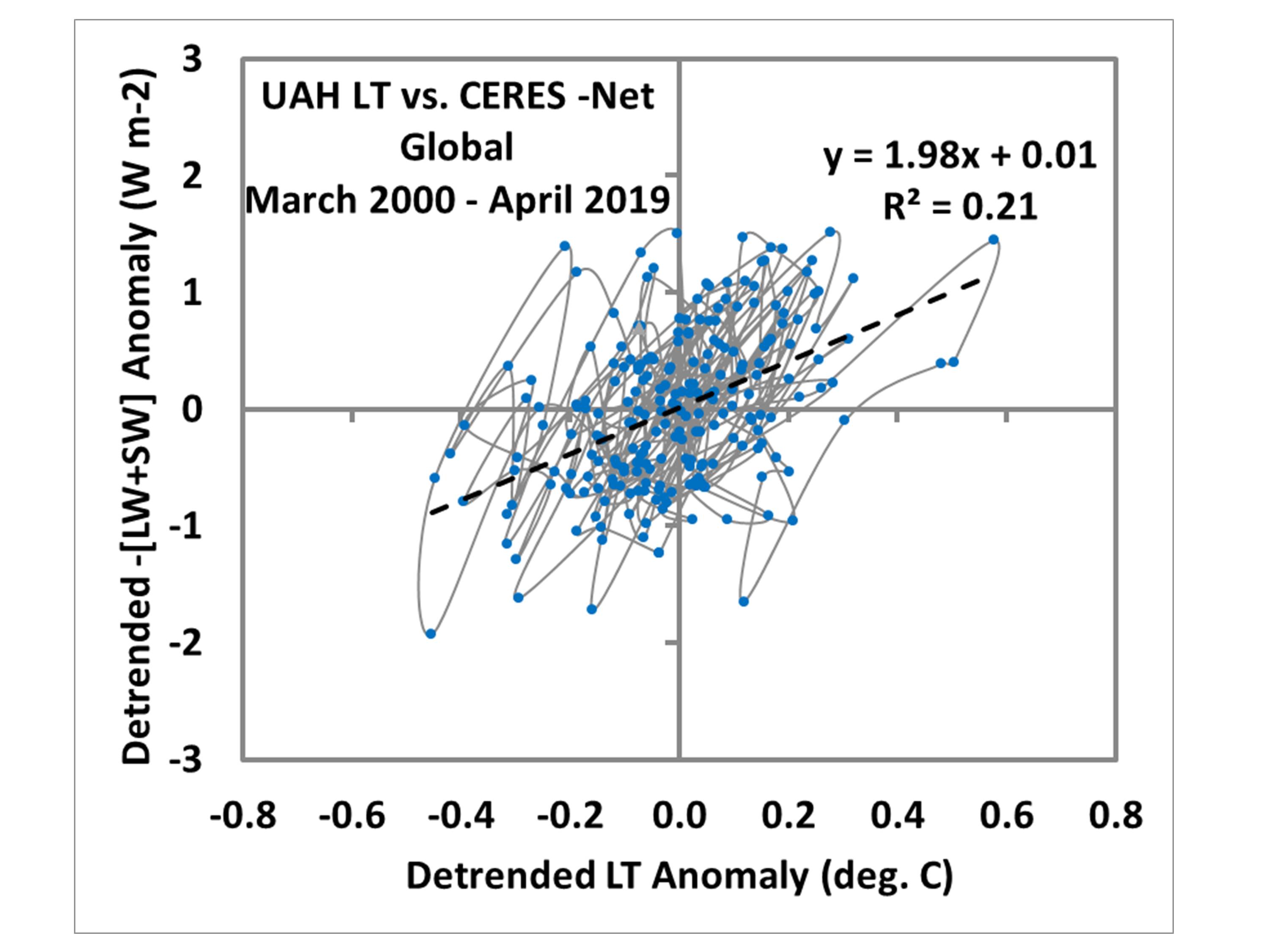
Note I have connected the data dots in chronological order. We see than “on average” (from the regression line) there appears to be about 2 W/m2 of energy lost per degree of warming of the lower troposphere. I say “appears” because some of the radiative variability in that plot is not due to feedback, and it decorrelates the data leading to uncertainty in the slope of the regression line, which we would like to be an estimate of the net feedback parameter.
This contaminating effect of internal radiative forcing can be demonstrated with a simple zero-dimensional time-dependent forcing-feedback model of temperature change of a swamp ocean:
Cp[dT(t)/dt] = F(t) – λ [dT(t)]
where the left side is the change in heat content of the swamp ocean with time, and on the right side F is all of the radiative and non-radiative forcings of temperature change (in W/m2) and λ is the net feedback parameter, which multiplies the temperature change (dT) from an assumed energy equilibrium state.
While this is probably the simplest time-dependent model you can create of the climate system, it shows behavior that we see in the climate system. For example, if I make time series of low-pass filtered random numbers about zero to represent the known time scales of intraseasonal oscillations and El Nino/La Nina, and add in another time series of low-pass filtered “internal radiative forcing”, I can roughly mimic the behavior seen in Fig. 1.
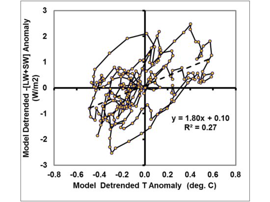
Now, the key issue for feedback diagnosis is that even though the regression line in Fig. 2 has a slope of 1.8 W m-2 K-1, the feedback I specified in the model run was 4 W m-2 K-1. Thus, if I had interpreted that slope as indicating the sensitivity of the simple model climate system, I would have gotten 2. 1 deg. C, when in fact the true specified sensitivity was only 0.9 deg. C (assuming 2XCO2 causes 3.7 W m-2 of radiative forcing).
This is just meant to demonstrate how internal radiative variability in the climate system corrupts the diagnosis of feedback from observational data, which is also a conclusion of the newer published studies referenced above.
And, as I have mentioned above, even if we can diagnose feedbacks from such short term variations in the climate system, we have no guarantee that they also determine (or are even related to) the long-term sensitivity to increasing CO2.
So (with the exception of studies like L&C) be prepared for increased reliance on climate models to tell us how sensitive the climate system is.


