Archive for 2021

An Earth Day Reminder: “Global Warming” is Only ~50% of What Models Predict

Thursday, April 22nd, 2021

The claim by the Biden Administration that climate change has placed us in a moment of “profound crisis” ignores the fact that the energy policy changes being promoted are based upon computer model simulations which have produced average warming rates at least DOUBLE those observed in the last 40+ years.

Just about every climate claim made by politicians, and even many vocal scientists, has been either an exaggeration or a lie.

While it is easy for detractors of what I will show to claim I am in the scientific minority (true), or that I am a climate denier (not true; I do not deny some level of human-caused warming), the fact is that the “official” observations in recent decades are in disagreement with the “official” climate models being promoted for the purposes of implementing expensive, economically-damaging, and poverty-worsening energy policies.

Global Ocean Temperatures are Warming at Only ~50% the Rate of Climate Model Projections

Today’s example comes from global-average sea surface temperatures. The oceans provide our best gauge of how fast extra energy is accumulating in the climate system. Since John Christy and I are working on a project that explains global ocean temperatures since the late 1800s with a 1D climate model, I thought I would show you just how the observations are comparing to climate models simulations.

The plot below (Fig. 1) shows the monthly global (60N-60S) average ocean surface temperature variations since 1979 for 68 model simulations from 13 different climate models. The 42 years of observations we now have since 1979 (bold black line) shows that warming is occurring much more slowly than the average climate model says it should have.

Fig. 1. 68 CMIP6 climate model simulations of global average sea surface temperature (relative to the 5 year average, 1979-1983), and compared to observations from the ERSSTv5 dataset.

In terms of the linear temperature trends since 1979, Fig. 2 shows that 2 of the top-cited ocean temperature datasets have warming trends near the bottom of the range of climate model simulations.

Fig. 2. Linear temperature trends, 1979-2020, for the various model and observational datasets in Fig. 1, plus the HadSST3 observational record.

Deep Ocean Warming Could Be Mostly Natural

A related issue is how much the deep oceans are warming. As I have mentioned before, the (inarguable) energy imbalance associated with deep-ocean warming in recent decades is only about 1 part (less than 1 Watt per sq. m) in 300 of the natural energy flows in the climate system.

This is a very tiny energy imbalance in the climate system. We know NONE of the natural energy flows to that level of accuracy.

What that means is that global warming could be mostly natural, and we would not even know it.

I’m not claiming that is the case. I am merely pointing out the level of faith that is involved in the adjustments made to climate models, which necessarily produce warming due to increasing CO2 because those models simply assume that there is no other source of warming.

Yes, more CO2 must produce some warming. But the amount of warming makes all the difference to global energy policies.

Seldom is the public ever informed of these glaring discrepancies between basic science and what politicians and pop-scientists tell us.

Why does it matter?

It matters because there is no Climate Crisis. There is no Climate Emergency.

Yes, irregular warming is occurring. Yes, it is at least partly due to human greenhouse gas emissions. But seldom are the benefits of a somewhat warmer climate system mentioned, or the benefits of more CO2 in the atmosphere (which is required for life on Earth to exist).

But if we waste trillions of dollars (that’s just here in the U.S. — meanwhile, China will always do what is in the best interests of China) then that is trillions of dollars not available for the real necessities of life.

Prosperity will suffer, and for no good reason.

UAH Global Temperature Update for March 2021: -0.01 deg. C

Friday, April 2nd, 2021

The Version 6.0 global average lower tropospheric temperature (LT) anomaly for March, 2021 was -0.01 deg. C, down substantially from the February, 2021 value of +0.20 deg. C.

REMINDER: We have changed the 30-year averaging period from which we compute anomalies to 1991-2020, from the old period 1981-2010. This change does not affect the temperature trends.

Right on time, the maximum impact from the current La Nina is finally being felt on global tropospheric temperatures. The global average oceanic tropospheric temperature anomaly is -0.07 deg. C, the lowest since November 2013. The tropical (20N-20S) departure from average (-0.29 deg. C) is the coolest since June of 2012. Australia is the coolest (-0.79 deg. C) since August 2014.

The linear warming trend since January, 1979 remains at +0.14 C/decade (+0.12 C/decade over the global-averaged oceans, and +0.18 C/decade over global-averaged land).

Various regional LT departures from the 30-year (1991-2020) average for the last 15 months are:

YEAR MO GLOBE NHEM. SHEM. TROPIC USA48 ARCTIC AUST 
2020 01 0.42 0.44 0.41 0.52 0.57 -0.22 0.41
2020 02 0.59 0.74 0.45 0.63 0.17 -0.27 0.20
2020 03 0.35 0.42 0.28 0.53 0.81 -0.96 -0.04
2020 04 0.26 0.26 0.25 0.35 -0.70 0.63 0.78
2020 05 0.42 0.43 0.41 0.53 0.07 0.83 -0.20
2020 06 0.30 0.29 0.30 0.31 0.26 0.54 0.97
2020 07 0.31 0.31 0.31 0.28 0.44 0.26 0.26
2020 08 0.30 0.34 0.26 0.45 0.35 0.30 0.25
2020 09 0.40 0.41 0.39 0.29 0.69 0.24 0.64
2020 10 0.38 0.53 0.22 0.24 0.86 0.95 -0.01
2020 11 0.40 0.52 0.27 0.17 1.45 1.09 1.28
2020 12 0.15 0.08 0.22 -0.07 0.29 0.43 0.13
2021 01 0.12 0.34 -0.09 -0.08 0.36 0.49 -0.52
2021 02 0.20 0.32 0.08 -0.14 -0.66 0.07 -0.27
2021 03 -0.01 0.12 -0.14 -0.29 0.59 -0.79 -0.79

The full UAH Global Temperature Report, along with the LT global gridpoint anomaly image for March, 2021 should be available within the next few days here.

The global and regional monthly anomalies for the various atmospheric layers we monitor should be available in the next few days at the following locations:

Lower Troposphere: http://vortex.nsstc.uah.edu/data/msu/v6.0/tlt/uahncdc_lt_6.0.txt
Mid-Troposphere: http://vortex.nsstc.uah.edu/data/msu/v6.0/tmt/uahncdc_mt_6.0.txt
Tropopause: http://vortex.nsstc.uah.edu/data/msu/v6.0/ttp/uahncdc_tp_6.0.txt
Lower Stratosphere: http://vortex.nsstc.uah.edu/data/msu/v6.0/tls/uahncdc_ls_6.0.txt

UAH Global Temperature Update for February 2021: +0.20 deg. C

Wednesday, March 3rd, 2021

The Version 6.0 global average lower tropospheric temperature (LT) anomaly for February, 2021 was +0.20 deg. C, up from the January, 2021 value of +0.12 deg. C.

REMINDER: We have changed the 30-year averaging period from which we compute anomalies to 1991-2020, from the old period 1981-2010. This change does not affect the temperature trends.

The linear warming trend since January, 1979 remains at +0.14 C/decade (+0.12 C/decade over the global-averaged oceans, and +0.18 C/decade over global-averaged land).

Various regional LT departures from the 30-year (1991-2020) average for the last 14 months are:

YEAR MO GLOBE NHEM. SHEM. TROPIC USA48 ARCTIC AUST 
2020 01 0.42 0.44 0.41 0.52 0.57 -0.22 0.41
2020 02 0.59 0.74 0.45 0.63 0.17 -0.27 0.20
2020 03 0.35 0.42 0.28 0.53 0.81 -0.96 -0.04
2020 04 0.26 0.26 0.25 0.35 -0.70 0.63 0.78
2020 05 0.42 0.43 0.41 0.53 0.07 0.83 -0.20
2020 06 0.30 0.29 0.30 0.31 0.26 0.54 0.97
2020 07 0.31 0.31 0.31 0.28 0.44 0.26 0.26
2020 08 0.30 0.34 0.26 0.45 0.35 0.30 0.25
2020 09 0.40 0.41 0.39 0.29 0.69 0.24 0.64
2020 10 0.38 0.53 0.22 0.24 0.86 0.95 -0.01
2020 11 0.40 0.52 0.27 0.17 1.45 1.09 1.28
2020 12 0.15 0.08 0.22 -0.07 0.29 0.43 0.13
2021 01 0.12 0.34 -0.09 -0.08 0.36 0.49 -0.52
2021 02 0.20 0.32 0.08 -0.14 -0.66 0.07 -0.27

The full UAH Global Temperature Report, along with the LT global gridpoint anomaly image for February, 2021 should be available within the next few days here.

The global and regional monthly anomalies for the various atmospheric layers we monitor should be available in the next few days at the following locations:

Lower Troposphere: http://vortex.nsstc.uah.edu/data/msu/v6.0/tlt/uahncdc_lt_6.0.txt
Mid-Troposphere: http://vortex.nsstc.uah.edu/data/msu/v6.0/tmt/uahncdc_mt_6.0.txt
Tropopause: http://vortex.nsstc.uah.edu/data/msu/v6.0/ttp/uahncdc_tp_6.0.txt
Lower Stratosphere: http://vortex.nsstc.uah.edu/data/msu/v6.0/tls/uahncdc_ls_6.0.txt

A Tribute to Rush Limbaugh

Wednesday, February 17th, 2021

As most you you know by now, Rush Limbaugh’s death from cancer was announced this morning. I suspected he would work right up to the end, and we would learn of his death when we least expected it. That was just Rush.

I don’t know when I started listening to him. I suspect it wasn’t long after his radio show became nationally syndicated in 1988. Like many of his life-long listeners, Rush was able to articulate things we were feeling at the time, but could not express very well.

As a tribute, I thought I would share some personal anecdotes about the man. There are so many things that his detractors get wrong.

It’s been over 10 years since I called into the show to talk about global warming. I wanted to support his views at the time. It was late in the 3-hour show that day, and he liked what I was saying, and asked if I could continue the conversation the next day.

They investigated my background overnight, and the next day he was excited to have an actual climate scientist on his side. That night we had a long e-mail conversation talking about how similar our backgrounds were growing up.

Within days he was calling me the “Chief Climatologist of the EIB Network”. An unpaid position, but he knew that mentioning my name on the radio was plenty payment enough; it led to many speaking opportunities in the years that followed. He provided me with his “super-secret” email address, and that’s how we would correspond from then on.

He immediately suggested I write my first book, and when it came out he plugged it on the show quite a few times. Within a couple weeks, his influence got the book on the NYT bestsellers list. When I told him the news, he had a typically funny response, “Watch out, Oprah!”

Over the last 10 years, he has always read my emails to him, and responded when appropriate. I could usually tell when it was something he would use on the air (and it was usually not related to climate). It took years before I got used to the idea that he was actually interested in what I had to say.

Not long after all this started, my family and I were visiting my daughter who was in law school in Miami, and Rush found out I was in the area. He invited us over to his house in Palm Beach on a Saturday, where his extended Missouri family was visiting for an annual sports weekend for a Missouri football game. Rush was a very gracious host, and his family and relatives are very friendly. He showed me around his palatial estate, showed me how his new cochlear implant worked, and gave me a tour of his climate-controlled cigar room. I was struck by how “average” of a guy he was on a personal level.

But my favorite memory of that visit was of David Limbaugh and my daughter (the law student) having a discussion about law while standing around the pool table. Rush was listening in (he would stroll from room to room to make sure all of his guests were being taken care of).

I was marveling at the whole experience: here was my daughter discussing law with David Limbaugh while Rush listened. I will never forget the surreal feeling I had in that moment.

He then entered the conversation (I don’t recall the specific subject) to explain about how the Bush administration had sent people down to Palm Beach more than once to change his mind on some issue. But he wouldn’t budge.

But that was Rush. He wasn’t a ‘political’ animal in the usual sense. He had specific conservative principles, and if the current Republican president violated them, Rush would not hesitate to call them on it.

Rush was the same person, on the air and off the air.

In the intervening years I would have hundreds of discussions with Rush, usually not on climate-related issues. I always marveled at his boundless energy… he always took time to find out what I wanted to say to him. Several times he would remember things I told him that I had forgotten I had told him!. Once I asked him, “How do you remember so much stuff?”. His silly answer was, “It’s the booze”.

Rush had a a unique combination of talents that probably won’t come together again. In addition to his unabashed conservativism, he could articulate those principles in a way that resonated with his listeners. He had a quick mind, perfect timing on the radio, a great radio voice, and he knew how to run a business. He had a great sense of humor; many of Paul Shanklin’s parody songs came from Rush’s ideas, and one even came from me, and one from my wife. I also gave him some advice on how to make the show better (something that I told him was confusing for listeners), which he actually took and implemented.

But the most important talent that distinguished Rush from the pack of radio personalities who sought to emulate his success was that he was genuinely kind to his callers, even if they disagreed with him. He let them speak. He praised them when there was merit to the points they were making, even if it seemed to be a stretch to praise them. Every liberal viewpoint that was called into the show was used as a teachable moment.

We are sorry we lost you so early, Rush.

Well done.

Urban Heat Island Effects on U.S. Temperature Trends, 1973-2020: USHCN vs. Hourly Weather Stations

Thursday, February 11th, 2021

SUMMARY: The Urban Heat Island (UHI) is shown to have affected U.S. temperature trends in the official NOAA 1,218-station USHCN dataset. I argue that, based upon the importance of quality temperature trend calculations to national energy policy, a new dataset not dependent upon the USHCN Tmax/Tmin observations is required. I find that regression analysis applied to the ISD hourly weather data (mostly from airports)  between many stations’ temperature trends and local population density (as a UHI proxy) can be used to remove the average spurious warming trend component due to UHI. Use of the hourly station data provides a mostly USHCN-independent measure of the U.S. warming trend, without the need for uncertain time-of-observation adjustments. The resulting 311-station average U.S. trend (1973-2020), after removal of the UHI-related spurios trend component, is about +0.13 deg. C/decade, which is only 50%  the USHCN trend of +0.26 C/decade. Regard station data quality, variability among the raw USHCN station trends is 60% greater than among the trends computed from the hourly data, suggesting the USHCN raw data are of a poorer quality. It is recommended that an de-urbanization of trends should be applied to the hourly data (mostly from airports) to achieve a more accurate record of temperature trends in land regions like the U.S. that have a sufficient number of temperature data to make the UHI-vs-trend correction.

The Urban Heat Island: Average vs. Trend Effects

In the last 50 years (1970-2020) the population of the U.S. has increased by a whopping 58%. More people means more infrastructure, more energy consumption (and waste heat production), and even if the population did not increase, our increasing standard of living leads to a variety of increases in manufacturing and consumption, with more businesses, parking lots, air conditioning, etc.

As T.R. Oke showed in 1973 (and many others since), the UHI has a substantial effect on the surface temperatures in populated regions, up to several degrees C. The extra warmth comes from both waste heat and replacements of cooler vegetated surfaces with impervious and easily heated hard surfaces. The effects can occur on many spatial scales: a heat pump placed too close to the thermometer (a microclimate effect) or a large city with outward-spreading suburbs (a mesoscale effect).

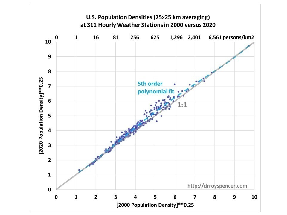
In the last 20 years (2000 to 2020) the increase in population has been largely in the urban areas, with no average increase in rural areas. Fig. 1 shows this for 311 hourly weather station locations that have relatively complete weather data since 1973.

Fig. 1. U.S. population increases around hourly weather stations have been in the more populated areas (except for mostly densely populated ones), with no increase in rural areas.

This might argue for only using rural data for temperature trend monitoring. The downside is that there are relatively few station locations which have population densities less than, say, 20 persons per sq. km., and so the coverage of the United States would be pretty sparse.

What would be nice is that if the UHI effect could be removed on a regional basis based upon how the average warming trends increase with population density. (Again, this is not removal of the average difference in temperature between rural and urban areas, but the removal of spurious temperature trends due to UHI effects).

But does such a relationship even exist?

UHI Effects on the USHCN Temperature Trends (1973-2020)

The most-cited surface temperature dataset for monitoring global warming trends in the U.S. is the U.S. Historical Climatology Network (USHCN). The dataset has a fixed set of 1,218 stations which have records extending back over 100 years. Because most of the stations’ data consist of daily maximum and minimum temperatures (Tmax and Tmin) measured at a single time daily, and that time of observation (TOBs) changed around 1960 from the late afternoon to the early morning (discussion here), there was a TOBs-related temperature bias that occurred, which is somewhat uncertain in magnitude but still must be adjusted for.

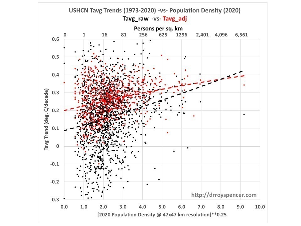
NOAA makes available both the raw unadjusted, and adjusted (TOBs & spatial ‘homogenization’) data. The following plot (Fig. 2) shows how both of the datasets’ station temperature trends are correlated with the population density, which should not be the case if UHI effects have been removed from the trends.

Fig.2. USHCN station temperature trends are correlated with population density, which should not be the case if the Urban Heat Island effect on trends has been removed.

Any UHI effect on temperature trends would be difficult to remove through NOAA’s homogenization procedure alone. This is because, if all stations in a small area, both urban and rural, are spuriously warming from UHI effects, then that signal would not be removed because it is also what is expected for global warming. ‘Homogenization’ adjustments can theoretically make the rural and urban trends look the same, but that does not mean the UHI effect has been removed.

Instead, one must examine the data in a manner like that in Fig. 2, which reveals that even the adjusted USHCN data (red dots) still have about a 30% overestimate of U.S. station-average trends (1973-2020) if we extrapolate a regression relationship (red dashed line, 2nd order polynomial fit) to zero population density. Such an analysis, however, requires many stations (thus large areas) to measure the average effect. It is not clear just how many stations are required to obtain a robust signal. The greater the number of stations needed, the larger the regional area required.

U.S. Hourly Temperature Data as an Alternative to USHCN

There are many weather stations in the U.S. which are (mostly) not included in the USHCN set of 1,218 stations. These are the operational  hourly weather stations operated by NWS, FAA, and other agencies, and which provide most of the data the National Weather Service reports to you. The data are included in the multi-agency Integrated Surface Database (ISD) archive.

The data archive is quite large, since it has (up to) hourly resolution data (higher with ‘special’ observations during changing weather) and many weather variables (temperature, dewpoint, wind, air pressure, precipitation) for many thousands of stations around the world. Many of the stations (at least in the U.S.) are at airports.

In the U.S., most of these measurements and their reporting are automated now, with the AWOS and ASOS systems.

This map shows all of the stations in the archive, although many of these will not have full records for whatever decades of time are of interest.

Fig. 3. Locations of ISD surface weather data quality-controlled and stored at NOAA.

The advantage of these data, at least in the United States, is that the equipment is maintained on a regular basis. When I worked summers at a National Weather Service office in Michigan, there was a full-time ‘met-tech’ who maintained and adjusted all of the weather-measuring equipment. 

Since the observations are taken (nominally) at the top of the hour, there is no uncertain TOBs adjustment necessary as with the USHCN daily Tmax/Tmin data.

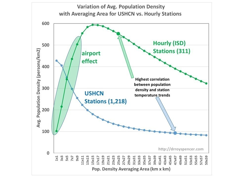
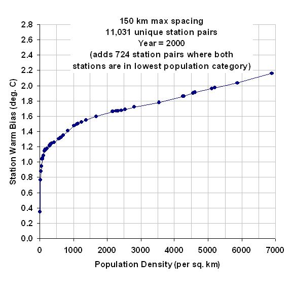
The average population density environment is markedly different between the ISD (‘hourly’) stations and the USHCN stations, as is shown in Fig. 4.

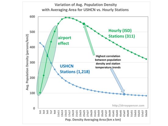
Fig. 4. The dependence of U.S. weather station population density on averaging area is markedly different between 1,218 USHCN and 311 high-quality ISD (‘hourly’) stations, mainly due to the measurement of the hourly data at “uninhabited” airports to support aviation safety.

In Fig. 4 we see that the population density in the immediate vicinity of the ISD stations averages only 100 people in the immediate 1 sq. km area since no one ‘lives’ at the airport, but then increases substantially with averaging area since airports exist to serve population centers.

In contrast, the USHCN stations have their highest population density right in the vicinity of the weather station (over 400 persons in the first sq. km), which then drops off with distance away from the station location.

How such differences affect the magnitude of UHI-dependent spurious warming trends is unknown at this point.

UHI Effects on the Hourly Temperature Data

I have analyzed the U.S. ISD data for the lower-48 states for the period 1973-2020. (Why 1973? Because many of the early records were on paper, and at hourly time resolution, that represents a lot of manual digitizing. Apparently, 1973 is as far back as many of those stations data were digitized and archived).

To begin with, I am averaging only the 00 UTC and 12 UTC temperatures (approximately the times of maximum and minimum temperatures in the United States). I required those twice-daily measurements to be reported on at least 20 days in order for a month to be considered for inclusion, and then at least 10 of 12 months from a station to have good data for a year of that station’s data to be stored.

Then, for temperature trend analysis, I required that 90% of the years 1973-2020 to have data, including the first 2 years (1973, 1974) and the last 2 years (2019-2020), since end years can have large effects on trend calculations.

The resulting 311 stations have an 8.7% commonality with the 1,218 USHCN stations. That is, only 8.7% of the (mostly-airport) stations are also included in the 1,218-station USHCN database, so the two datasets are mostly (but not entirely) independent.

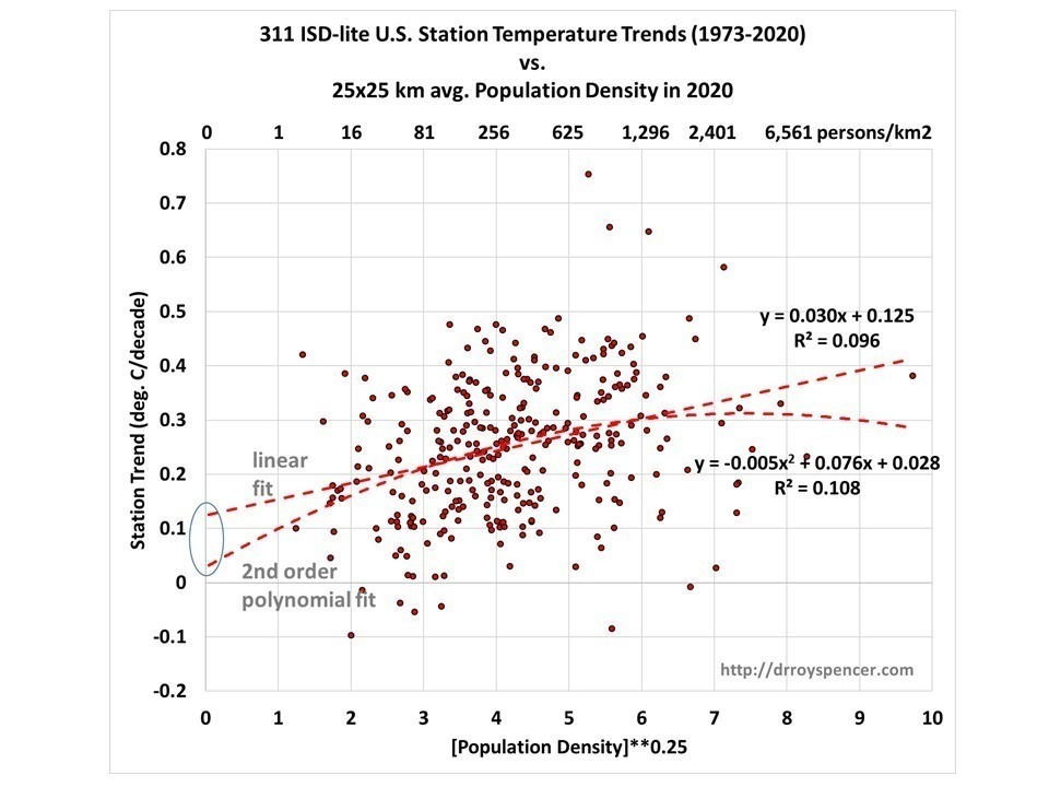
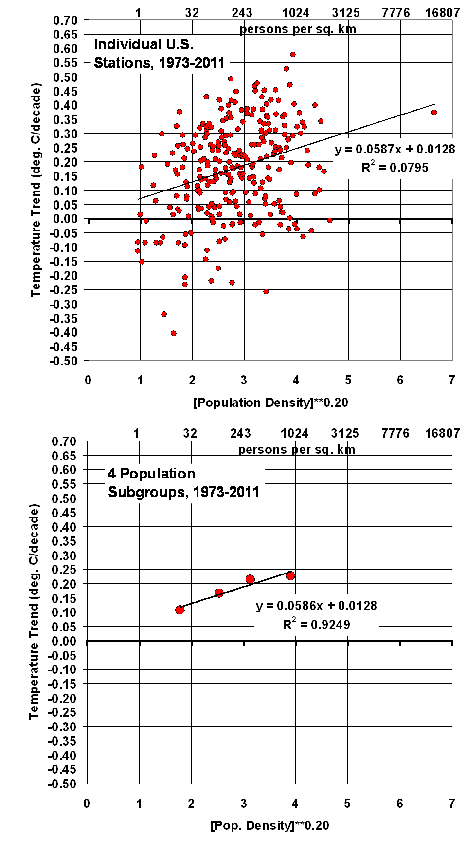
I then plotted the Fig. 2 equivalent for the ISD stations (Fig. 5).

Fig. 5. As in Fig. 2, but for the ISD (mostly airport) station trends for the average of daily 00 and 12 UTC temperatures. Where the regression lines intercept the zero population axis is an estimate of the U.S. temperature trend during 1973-2020 with spurious UHI trend effects removed.

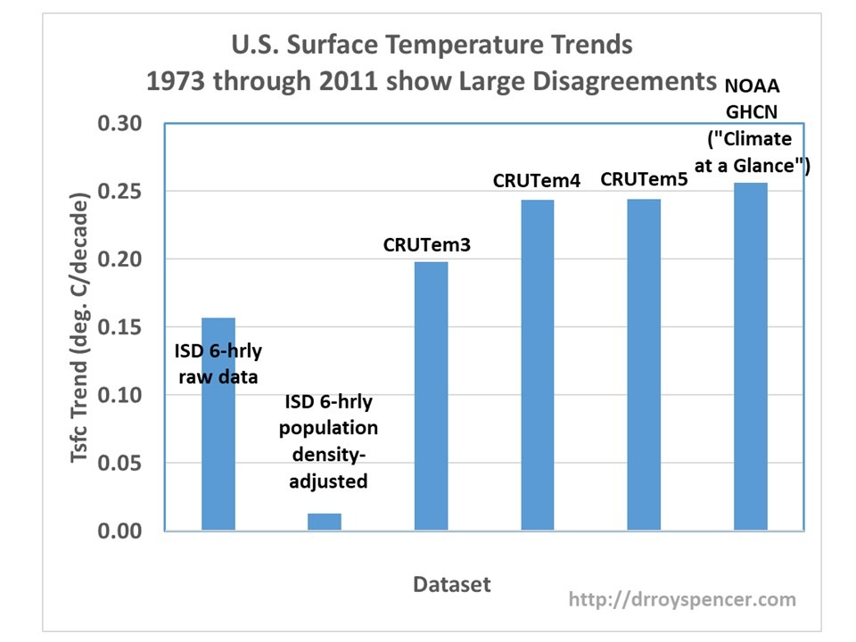
We can see for the linear fit to the data, extrapolation of the line to zero population density gives a 311-station average warming trend of +0.13 deg. C/decade.

Significantly, this is only 50% of the USHCN 1,218-station official TOBs-adjusted, homogenized average trend of +0.26 C/decade.

It is also significant that this 50% reduction in the official U.S temperature trend is very close to what Anthony Watts and co-workers obtained in their 2015 analysis using the very best-sited USHCN stations.

I also include the polynomial fit in Fig. 5, since my use of the fourth root of the population density is not meant to perfectly capture the nonlinearity of the UHI effect, and some nonlinearity can be expected to remain. In that case, the extrapolated warming trend at zero population density is close to zero. But for the purpose of the current discussion, I will conservatively use the linear fit in Fig. 5. (The logarithm of the population density is sometimes also used, but is not well behaved as the population approaches zero.)

Evidence that the raw ISD station trends are of higher quality than those from UHCN is in the standard deviation of those trends:

Std. Dev. of 1,218 USHCN (raw) trends = +0.205 deg. C/decade

Std. Dev. of 311 ISD (‘hourly’) trends = +0.128 deg. C/decade

Thus, the variation in the USHCN raw trends is 60% greater than the variation in the hourly station trends, suggesting the airport trends have fewer time-changing spurious temperature influences than do the USHCN station trends.

Conclusions

For the period 1973-2020:

  1. The USHCN homogenized data still have spurious warming influences related to urban heat island (UHI) effects. This has exaggerated the global warming trend for the U.S. as a whole. The magnitude of that spurious component is uncertain due to the black-box nature of the ‘homogenization’ procedure applied to the raw data.
  2. An alternative analysis of U.S. temperature trends from a mostly independent dataset from airports suggests that the U.S. UHI-adjusted average warming trend (+0.13 deg. C/decade) might be only 50% of the official USHCN station-average trend (+0.26 deg. C/decade).
  3. The raw USHCN trends have 60% more variability than the raw airport trends, suggesting higher quality of the routinely maintained airport weather data.

Future Work

This is an extension of work I started about 8 years ago, but never finished. John Christy and I are discussing using results based upon this methodology to make a new U.S. surface temperature dataset which would be updated monthly.

I have only outlined the very basics above. One can perform similar calculations in sub-regions (I find the western U.S. results to be similar to the eastern U.S. results). Also, the results would probably have a seasonal dependence in which case that should be calculated by calendar month.

Of course, the methodology could also be applied to other countries.

UAH Global Temperature Update for January 2021: +0.12 deg. C (new base period)

Tuesday, February 2nd, 2021

The Version 6.0 global average lower tropospheric temperature (LT) anomaly for January, 2021 was +0.12 deg. C, down a little from the December, 2020 value of +0.15 deg. C. NOTE: We have changed the 30-year averaging period from which we compute anomalies to 1991-2020, from the old period 1981-2010. This change does not affect the temperature trends.

The linear warming trend since January, 1979 remains at +0.14 C/decade (+0.12 C/decade over the global-averaged oceans, and +0.18 C/decade over global-averaged land).

Various regional LT departures from the 30-year (1991-2020) average for the last 13 months are:

YEAR MO GLOBE NHEM. SHEM. TROPIC USA48 ARCTIC AUST 
2020 01 0.42 0.44 0.41 0.52 0.57 -0.22 0.41
2020 02 0.59 0.74 0.45 0.63 0.17 -0.27 0.20
2020 03 0.35 0.42 0.28 0.53 0.81 -0.96 -0.04
2020 04 0.26 0.26 0.25 0.35 -0.70 0.63 0.78
2020 05 0.42 0.43 0.41 0.53 0.07 0.83 -0.20
2020 06 0.30 0.29 0.30 0.31 0.26 0.54 0.97
2020 07 0.31 0.31 0.31 0.28 0.44 0.26 0.26
2020 08 0.30 0.34 0.26 0.45 0.35 0.30 0.25
2020 09 0.40 0.41 0.39 0.29 0.69 0.24 0.64
2020 10 0.38 0.53 0.22 0.24 0.86 0.94 -0.01
2020 11 0.40 0.52 0.27 0.17 1.45 1.09 1.28
2020 12 0.15 0.08 0.22 -0.07 0.29 0.43 0.13
2021 01 0.12 0.34 -0.09 -0.08 0.36 0.49 -0.52

The full UAH Global Temperature Report, along with the LT global gridpoint anomaly image for January, 2021 should be available within the next few days here.

The global and regional monthly anomalies for the various atmospheric layers we monitor should be available in the next few days at the following locations:

Lower Troposphere: http://vortex.nsstc.uah.edu/data/msu/v6.0/tlt/uahncdc_lt_6.0.txt
Mid-Troposphere: http://vortex.nsstc.uah.edu/data/msu/v6.0/tmt/uahncdc_mt_6.0.txt
Tropopause: http://vortex.nsstc.uah.edu/data/msu/v6.0/ttp/uahncdc_tp_6.0.txt
Lower Stratosphere: http://vortex.nsstc.uah.edu/data/msu/v6.0/tls/uahncdc_ls_6.0.txt

Could Recent U.S. Warming Trends be Largely Spurious?

Friday, January 29th, 2021

Several lines of evidence suggest observed warming trends are not nearly as large as what you have been told.

It’s been almost eight years since I posted results on my analysis of the global Integrated Surface Database (ISD) temperature data. Despite finding evidence that urbanization effects on temperature measurements have not been removed from official land temperature datasets, I still refer people to the official products (e.g. from NOAA GHCN, HadCRUT, etc.). This is because I never published any results from my analysis.

But I’ve started thinking again about the question, Just how much warming has there been in recent decades (say, the last 50 years)? The climate models suggest that this should have been the period of most rapid warming, due to ever-increasing atmospheric CO2 combined with a reduction in aerosol pollution. Since those models are the basis for proposed changes in energy policy, it is important that the observations to which they are compared be trustworthy.

A Review of the Diagnosed Urban Heat Island Effect

The official datasets of land surface temperature are (we are told) already adjusted for Urban Heat Island (UHI) effects. But as far as I know, it has never been demonstrated that the spurious warming from urban effects have been removed. Making temperature trends be the same independent of urbanization does NOT mean urban warming effects have been removed. It could be that spurious warming has simply been spread around to the non-affected stations.

Back in 2010 I quantified the Urban Heat Island (UHI) effect, based upon the difference in absolute temperatures between closely-spaced neighboring stations having different population densities (PD). The ISD temperature data are not max/min (as in GHCN), but data taken hourly, with the longest-record stations reporting at just the 6-hourly synoptic times (00, 06, 12, 18 UTC). Because there were many more stations added to the global dataset in 1973, all of my analyses started then.

By using many station pairs from low to high population densities, I constructed the cumulative UHI effect as a function of population density. Here are the results from global data in the year 2000:

Fig. 1. Diagnosed average Urban Heat Island warming in 2000 from over 11,000 closely spaced station pairs having different population densities.

As can be seen, the largest warming effect with a change in population density occurs at the lowest population densities (not a new finding), with the most total warming at the highest population densities.

The Effect of Population Density on U.S. Station Temperature Trends

In 2012 I experimented with methods to removed the observed UHI effect in the raw ISD 6-hourly data using population density as a proxy. As you can see in the second of the two graphs below, the highest population density stations had ~0.25 C/decade warming trend, with a reduced warming trend as population density was reduced:

Fig. 2. U.S. surface temperature trends as a function of local population density at the station locations: top (raw), bottom (averages into 4 groups).

Significantly, extrapolating to zero population density would give essentially no warming in the United States during 1973-2011. As we shall see (below) official temperature datasets say this period had a substantial warming trend, consistent with the warming in the highest population density locations.

How can one explain this result other than, at least for the period 1973-2011, (1) spurious warming occurred at the higher population density stations, and (2) the evidence supports essentially no warming if there were no people (zero population density) to modify the microclimate around thermometer sites?

I am not claiming there has been no global warming (whatever the cause). I am claiming that there is evidence of spurious warming in thermometer data which must be removed.

Next, we will examine how well that effect has been removed.

How Does this Compare to the ‘Official’ Temperature Trends?

Since I performed these analyses almost 10 years ago, the ‘official’ temperature datasets have been adjusted several times. For the same period I analyzed 8-10 years years ago, look at how some of these datasets have increased the temperature trends (I used only CRUTem3 back then):

Fig. 3. U.S. surface temperature trend from different datasets.

The CRUTem3 data produce a trend reasonably close to the raw, unadjusted 6-hourly ISD-based data (the correlation of the two datasets’ monthly anomaly time series was 0.994). Note that the latest USHCN data in the above graph has the most warming, at +0.26 C/decade.

Note that this is about the same as the trend I get with the stations having the highest (rather than lowest) population density. Anthony Watts reported qualitatively similar results using different data back in 2015.

How in the world can the warming result from NOAA be reconciled with the (possible zero warming) results in Fig. 2? NOAA uses a complex homogenization procedure to make its adjustments, but it seems to me the the results in Fig. 2 suggest that their procedures might be causing spurious warming trends in the data. I am not the first to point this out; others have made the same claims over the years. I am simply showing additional quantitative evidence.

I don’t see how it can be a change in instrumentation, since both rural and urban stations changed over the decades from liquid-in-glass thermometers in Stevenson screens, to digital thermistors in small hygrothermometer enclosures, to the new automated ASOS measurement systems.

Conclusion

It seems to me that there remains considerable uncertainty in just how much the U.S. has warmed in recent decades, even among the established, official, ‘homogenized’ datasets. This has a direct impact on the “validation” of climate models relied upon by the new Biden Administration for establishing energy policy.

I would not be surprised if such problems exist in global land temperature datasets in addition to the U.S.

I’m not claiming I know how much it has (or hasn’t) warmed. Instead, I’m saying I am still very suspicious of existing official land temperature datasets.

Biden to End Fossil Fuel Subsidies: Like the Paris Agreement, it Will Make No Difference

Wednesday, January 27th, 2021

Joe Biden’s administration has made climate change one of its top priorities. Photographer: Doug Mills/The New York Times/Bloomberg

In what appears to be a never-ending string of ineffective efforts to force the public to use expensive, unreliable, intermittent, and not-widely-deployable renewable energy, the Biden Administration is issuing an executive order that (among other things) directs federal agencies to end fossil fuel subsidies.

Personally, I would not mind if all federal subsidies were ended, since all that subsidies do is put the government, rather than the consumer, in charge of what you spend your money on.

But federal subsidies on fossil fuels represent less that 3% of the revenues of the fossil fuel industry. This action will have essentially no impact on an economy that still runs on fossil fuels. That 3% will be voluntarily paid by the consumer, just directly rather than through subsidies.

In contrast, renewables currently enjoy 25 times the level of subsides per unit of energy produced as do fossil fuels, and the market penetration of EVs is still only 1.2%. One can see that massive government meddling in the energy market is the only way that people will — at least for the foreseeable future — “choose” renewables over fossil fuels.

So, while environmentalists might applaud Biden’s decision, the effect on the energy markets will be barely measurable, if at all.

You see, when it comes to global warming, modern environmentalism depends upon feelings over facts. Even if all CO2 emissions in the U.S. were to end, the impact on global temperatures by 2100 would be small. This is because the U.S. now produces less than 15% of the global total greenhouse gas emissions. The same is true if all countries abide by their commitments under the Paris Climate Agreement, which makes Biden’s rejoining that Agreement rather pointless. The effect of Paris is calculated to be a 0.2 deg. C reduction in warming by 2100, which is too small to measure over the next 80 years with temperature monitoring technologies currently in place.

Even the godfather of modern global warming alarmism, NASA’s James Hansen says the Paris Agreement is ineffective and a “fraud”, and that only massive taxation of (i.e. punishment for) using fossil fuels will make much difference.

To show just how much CO2 emissions will have to decrease to affect the atmospheric CO2 concentration, just look at what happened (or didn’t happen) last year. The U.S. Energy Information Agency (EIA) estimates that the economic downturn in 2020 produced only an 11% reduction in fossil fuel use. The resulting change in atmospheric CO2 concentration was unmeasurable:

The 11% reduction in global CO2 emissions in 2020 had no measurable impact on atmospheric CO2 concentrations at Mauna Loa, Hawaii.

Furthermore, while we nibble around the edges of the “carbon pollution” problem, China’s CO2 emissions continue to grow.

The U.S. has led the way in reducing CO2 emissions, mainly through a market-driven switch from coal to natural gas in recent years, China’s emissions continue to grow.

And while the “social cost of carbon” continues to be advanced as the justification for reducing CO2 emissions, no one wants to talk about the social benefits. For example, Nature loves the stuff. It is estimated that global agricultural productivity has increased by $3.5 Trillion from the extra CO2 in the atmosphere. It is well known that excessive cold kills far more people than excessive heat. There is no evidence that recent, modest global warming has caused a global-average increase in severe weather.

The claims by China that they will become “carbon neutral” by 2060 is just political posturing. One thing I have learned about China in recent decades is that their political culture is to say anything necessary to nominally appease other countries, and then do just the opposite if it suits their national interests. With over four times the population of the U.S., one can see why they would not want the U.S. (or any other county) dictating their behavior, especially as they continue to lift millions out of poverty.

Not unless the Biden Administration pushes for a massive increase in the taxation of fossil fuels, and then embraces either nuclear plant construction or widespread wind and solar projects to service a huge fleet of electric vehicles (currently at 1.2% of U.S. market penetration) will there be any substantial move away from fossil fuels.

Anything less will only falsely assuage fears rather than address facts.

Canada is Warming at Only 1/2 the Rate of Climate Model Simulations

Thursday, January 21st, 2021

As part of my Jan. 19 presentation for Friends of Science about there being no climate emergency, I also examined surface temperature in Canada to see how much warming there has been compared to climate models.

Canada has huge year-to-year variability in temperatures due to its strong continental climate. So, to examine how observed surface temperature trends compare to climate model simulations, you need many of those simulations, each of which exhibits its own large variability.

I examined the most recent 30-year period (1991-2020), using a total of 108 CMIP5 simulations from approximately 20 different climate models, and computed land-surface trends over the latitude bounds of 51N to 70N, and longitude bounds 60W to 130W, which approximately covers Canada. For observations, I used the same lat/lon bounds and the CRUTem5 dataset, which is heavily relied upon by the UN IPCC and world governments. All data were downloaded from the KNMI Climate Explorer.

First let’s examine the annual average temperature departures from the 1981-2010 average, for the average of the 108 model simulations compared to the observations. We see that Canada has been warming at only 50% the rate of the average of the CMIP5 models; the linear trends are +0.23 C/decade and +0.49 C/decade, respectively. Note that in 7 of the last 8 years, the observations have been below the average of the models.

Fig. 1. Yearly temperature departures 1991-2020 from the 1981-2010 mean in Canada in observations (blue) versus the average of 108 CMIP5 climate model simulations (red). The +/-1 standard deviation bars indicate the variability among the 108 individual model simulations.

Next, I show the individual models’ trends compared to the observed trends, with a histogram of the ranked values from the least warming to the most warming, 1991-2020.

Fig. 2. Ranked Canada surface temperature trends (1991-2020) for the 108 model simulations and the observations.

Note that the 93.5% of the model simulations have warmer temperature trends than the observations exhibit.

These results from Canada are generally consistent with the results I have found in the Midwest U.S. in the summertime, where the CMIP5 models warm, on average, 4 times faster than the observations (since 1970), and 6 times faster in a limited number of the newer CMIP6 model simulations.

Implications

The Paris Climate Accords, among other national and international efforts to reduce greenhouse gas emissions, assume warming estimates which are approximately the average of the various climate models. Thus, these results impact directly on those proposed energy policy decisions.

As you might be aware, proponents of those climate models often emphasize the general agreement between the models and observations over a long period of time, say since 1900.

But this is misleading.

We would expect little anthropogenic global warming signal to emerge from the noise of natural climate variability until (approximately) the 1980s. This is for 2 reasons: There was little CO2 emitted up through the 1970s, and even as the emissions rose after the 1940s the cooling effect of anthropogenic SO2 emissions was canceling out much of that warming. This is widely agreed to by climate modelers as well.

Thus, to really get a good signal of global warming — in both observations and models — we should be examining temperature trends since approximately the 1980s. That is, only in the decades since the 1980s should we be seeing a robust signal of anthropogenic warming against the background of natural variability, and without the confusion (and uncertainty) in large SO2 emissions in the mid-20th century.

And as each year passes now, the warming signal should grow slightly stronger.

I continue to contend that climate models are now producing at least twice as much warming as they should, probably due to an equilibrium climate sensitivity which is about 2X too high in the climate models. Given that the average CMIP6 climate sensitivity is even larger than in CMIP5 — approaching 4 deg. C — it will be interesting to see if the divergence between models and observations (which began around the turn of the century) will continue into the future.


This Tuesday, Jan. 19: My Friends of Science Society Livestream Talk: ‘Why There Is No Climate Emergency’

Friday, January 15th, 2021

On Tuesday evening, January 19, at 8 p.m. CST there will be a 30 minute livestream presentation where I cover the most important reasons why there is no climate emergency. I just reviewed the video and I am very satisfied with it.

In only 1/2 hour I cover what I consider to be the most important science issues, the disinformation campaign that spreads climate hysteria, some of the harm that will be caused by forcing expensive and unreliable renewable energy upon humanity, and the benefits of more CO2 in the atmosphere.

You can go to the FoS website for more information. The tickets are $15, and I will be doing a live Q&A after the event.