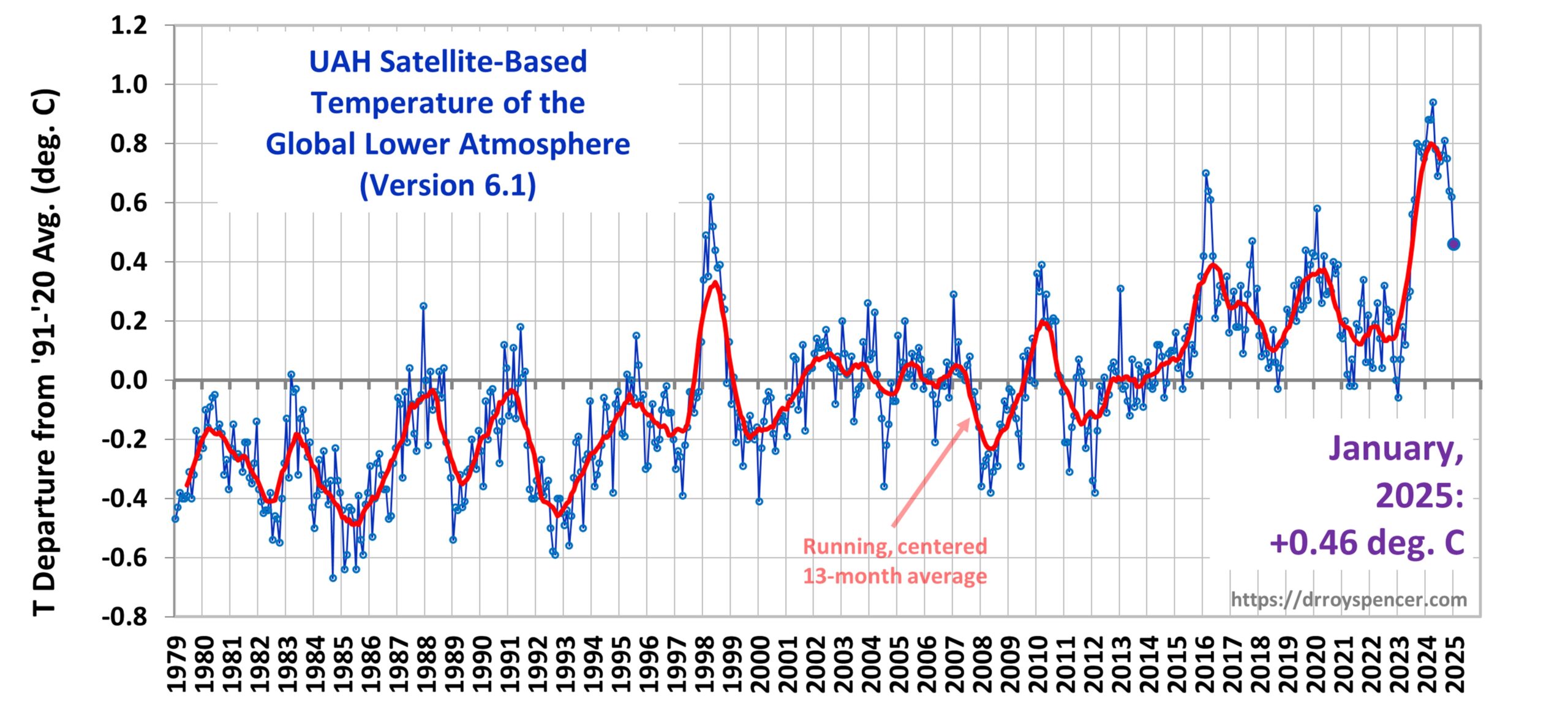
The Version 6.1 global average lower tropospheric temperature (LT) anomaly for February, 2025 was +0.50 deg. C departure from the 1991-2020 mean, up a little from the January, 2025 anomaly of +0.45 deg. C.
The Version 6.1 global area-averaged linear temperature trend (January 1979 through February 2025) remains at +0.15 deg/ C/decade (+0.22 C/decade over land, +0.13 C/decade over oceans).
The following table lists various regional Version 6.1 LT departures from the 30-year (1991-2020) average for the last 14 months (record highs are in red).
YEAR
MO
GLOBE
NHEM.
SHEM.
TROPIC
USA48
ARCTIC
AUST
2024
Jan
+0.80
+1.02
+0.58
+1.20
-0.19
+0.40
+1.12
2024
Feb
+0.88
+0.95
+0.81
+1.17
+1.31
+0.86
+1.16
2024
Mar
+0.88
+0.96
+0.80
+1.26
+0.22
+1.05
+1.34
2024
Apr
+0.94
+1.12
+0.77
+1.15
+0.86
+0.88
+0.54
2024
May
+0.78
+0.77
+0.78
+1.20
+0.05
+0.20
+0.53
2024
June
+0.69
+0.78
+0.60
+0.85
+1.37
+0.64
+0.91
2024
July
+0.74
+0.86
+0.61
+0.97
+0.44
+0.56
-0.07
2024
Aug
+0.76
+0.82
+0.70
+0.75
+0.41
+0.88
+1.75
2024
Sep
+0.81
+1.04
+0.58
+0.82
+1.31
+1.48
+0.98
2024
Oct
+0.75
+0.89
+0.61
+0.64
+1.90
+0.81
+1.09
2024
Nov
+0.64
+0.88
+0.41
+0.53
+1.12
+0.79
+1.00
2024
Dec
+0.62
+0.76
+0.48
+0.52
+1.42
+1.12
+1.54
2025
Jan
+0.45
+0.70
+0.21
+0.24
-1.06
+0.74
+0.48
2025
Feb
+0.50
+0.55
+0.45
+0.26
+1.04
+2.10
+0.87
The full UAH Global Temperature Report, along with the LT global gridpoint anomaly image for February, 2025, and a more detailed analysis by John Christy, should be available within the next several days here.
The monthly anomalies for various regions for the four deep layers we monitor from satellites will be available in the next several days at the following locations:
Today, the Washington Post is reporting the EPA Administrator is considering recommending to the White House that the EPA’s 2009 CO2 Endangerment Finding be rescinded. Let’s look at a few of the reasons why this might be a good thing to consider.
The Science
The science of human-caused climate change is much more uncertain that you have been led to believe. The globally-averaged surface temperature of Earth seems to have warmed by 1 deg. C or so in the last century. The magnitude of the warming remains uncertain with a 30% range in different thermometer-based datasets, and considerably weaker warming in global “reanalysis” datasets using all available data types. But whatever the level of warming, it might well be mostly human-caused.
But we don’t really know.
As I keep pointing out, the global energy imbalance caused by increasing human-caused CO2 emissions (yes, I believe we are the cause) is smaller than the accuracy with which we know natural energy flows in the climate system. This means recent warming could be mostly natural and we would never know it.
I’m not claiming that is the case, only that there are uncertainties in climate science that are seldom if ever discussed. The climate models that are the basis for future projections of climate change are adjusted (fudged?) so that increasing CO2 is the only cause of warming. The models themselves do not have all of the necessary physics (mostly due to cloud process uncertainties) to determine whether our climate system was in a state of equilibrium before CO2 was increasing. (And, no, I don’t believe the warming caused the oceans to outgas more CO2 — that effect is very small compared to the size of the human source).
As most readers here are aware, for many years I’ve been saying the science of “climate change” has been corrupted by big government science budgets, ideological worldview biases, and group-think. Even my career has depended upon Congress being convinced the issue is worthy of big budgets.
It is almost impossible for new science to be published in the peer-reviewed literature that in any way runs counter to the current narrative which states that humans are causing a “climate crisis” from our CO2 emissions, a natural consequence of fossil fuel burning. That “peer review” is now in the hands of climate scientists whose research careers depend upon continuing government funding. If the “problem” of global warming were to be much less than previously believed, funding for that research could dry up.
The most alarmist science papers are the ones that get all of the press, which then get exaggerated and misrepresented by the news media. As a result, the public has a very skewed perception of what scientists really know.
As Roger Pielke, Jr. has been pointing out for many years, even the IPCC’s official reports do not claim that our greenhouse gas emissions have caused changes in severe weather. Every severe weather event in the news is now dutifully tied in some inferential way to human causation, but with public opinion of mainstream news outlets at an all-time low, fewer and fewer people take those news reports seriously. Severe weather has always existed, and always will. Storm damages have increased only because of increasing infrastructure and everyone wanting to live on the coast.
And about the only, clear, long-term change I’m aware of is a 50% decline in strong to violent tornadoes since the 1950s.
But you would never know of any good climate news if your main source of information is Al Gore’s books, your favorite environmental think tank (that you contribute to so you can get their yearly calendar), or the mainstream media.
Costs vs. Benefits
If there was no cost to replacing fossil fuels with renewable sources of energy, I might be a little more supportive of regulations which choose winners and losers, rather than letting the marketplace decide. But everything humans do requires energy, and so human flourishing depends upon abundant and affordable energy. We in the developed world might have excess wealth to spend on pricey new forms of energy (although our rapidly increasing national debt argues we don’t have excess wealth to squander), but most of the world’s poor continue to struggle to pay for energy we have in relative abundance… if they even have access to it.
The 2009 Endangerment Finding
The Supreme Court has ruled that CO2 falls under the EPA’s Clean Air Act, and so EPA would need to regulate it if it was considered a threat to human health and welfare. Which it did in 2009.
But this “threat to human health and welfare” business cuts both ways.
For example, I could argue that most premature human deaths are caused, indirectly, by what we eat (or don’t eat). The incidence of obesity and related illnesses continues to rise. So, given the threat of food to human and welfare, why not just outlaw food? Food is a threat to human health and welfare, too.
Clearly we don’t do that because food is necessary for life. But so is CO2.
CO2 is required for photosynthesis, which in turn is required for the food chain on land and in the oceans. NASA-based satellite measurements since the 1980s have documented global greening from increasing CO2. It has been estimated global agricultural productivity has increased by trillions of dollars from crops growing better, with more drought resistance, in a CO2-enriched atmosphere.
I’ve read the technical support document for the 2009 EF. It is full of gloom and doom. Any benefits to more CO2 are downplayed while costs are trumpeted. Its authorship appears to have been heavily influenced by environmental activists, most of whom have their own agendas. Much of the science in it now sounds more like Al Gore’s original alarmist book Earth In The Balance (which referenced me, but couldn’t get my science contributions right) than a balanced assessment of the science of climate change.
Fifteen years since the 2009 Endangerment Finding, we now know much more. None of the scary scenarios originally predicted have actually come to pass, or at a minimum they were greatly exaggerated. Ten-year deadlines to “do something” about the “climate crisis” have come and gone since this mess started in the 1980s… a few times over. Even the IPCC (which only allows alarmist-leaning scientists to participate) has admitted it is unlikely we will experience significant changes in severe weather by the year 2100 that can be tied to increasing CO2.
It makes sense to now reconsider the Endangerment Finding. Let the free market (including consumer preferences) decide which forms of energy we use.
The Version 6.1 global average lower tropospheric temperature (LT) anomaly for January, 2025 was +0.46 deg. C departure from the 1991-2020 mean, down substantially from the December, 2024 anomaly of +0.62 deg. Most of this cooling was over the global oceans.
The Version 6.1 global area-averaged temperature trend (January 1979 through January 2025) remains at +0.15 deg/ C/decade (+0.22 C/decade over land, +0.13 C/decade over oceans).
The following table lists various regional Version 6.1 LT departures from the 30-year (1991-2020) average for the last 13 months (record highs are in red).
YEAR
MO
GLOBE
NHEM.
SHEM.
TROPIC
USA48
ARCTIC
AUST
2024
Jan
+0.80
+1.02
+0.58
+1.20
-0.19
+0.40
+1.12
2024
Feb
+0.88
+0.95
+0.81
+1.17
+1.31
+0.86
+1.16
2024
Mar
+0.88
+0.96
+0.80
+1.26
+0.22
+1.05
+1.34
2024
Apr
+0.94
+1.12
+0.77
+1.15
+0.86
+0.88
+0.54
2024
May
+0.78
+0.77
+0.78
+1.20
+0.05
+0.20
+0.53
2024
June
+0.69
+0.78
+0.60
+0.85
+1.37
+0.64
+0.91
2024
July
+0.74
+0.86
+0.61
+0.97
+0.44
+0.56
-0.07
2024
Aug
+0.76
+0.82
+0.70
+0.75
+0.41
+0.88
+1.75
2024
Sep
+0.81
+1.04
+0.58
+0.82
+1.31
+1.48
+0.98
2024
Oct
+0.75
+0.89
+0.61
+0.64
+1.90
+0.81
+1.09
2024
Nov
+0.64
+0.88
+0.41
+0.53
+1.12
+0.79
+1.00
2024
Dec
+0.62
+0.76
+0.48
+0.53
+1.42
+1.12
+1.54
2025
Jan
+0.46
+0.70
+0.21
+0.24
-1.06
+0.74
+0.48
The full UAH Global Temperature Report, along with the LT global gridpoint anomaly image for January, 2025, and a more detailed analysis by John Christy, should be available within the next several days here.
The monthly anomalies for various regions for the four deep layers we monitor from satellites will be available in the next several days at the following locations:
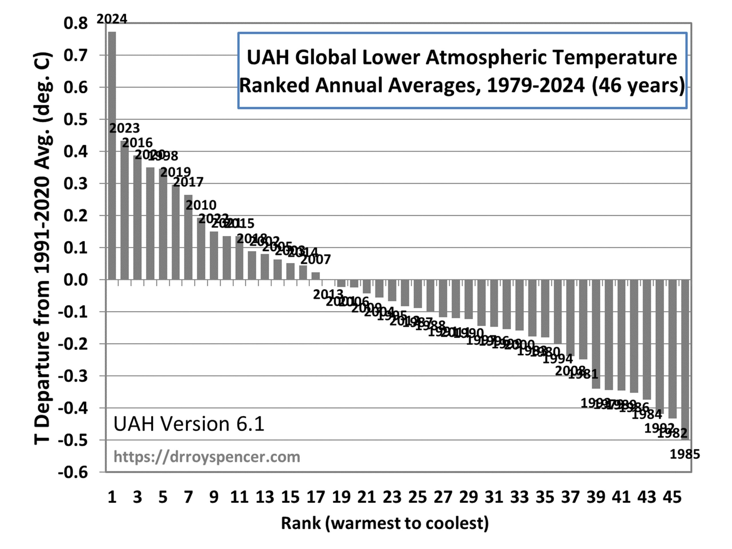
2024 Sets New Record for Warmest Year In Satellite Era (Since 1979)
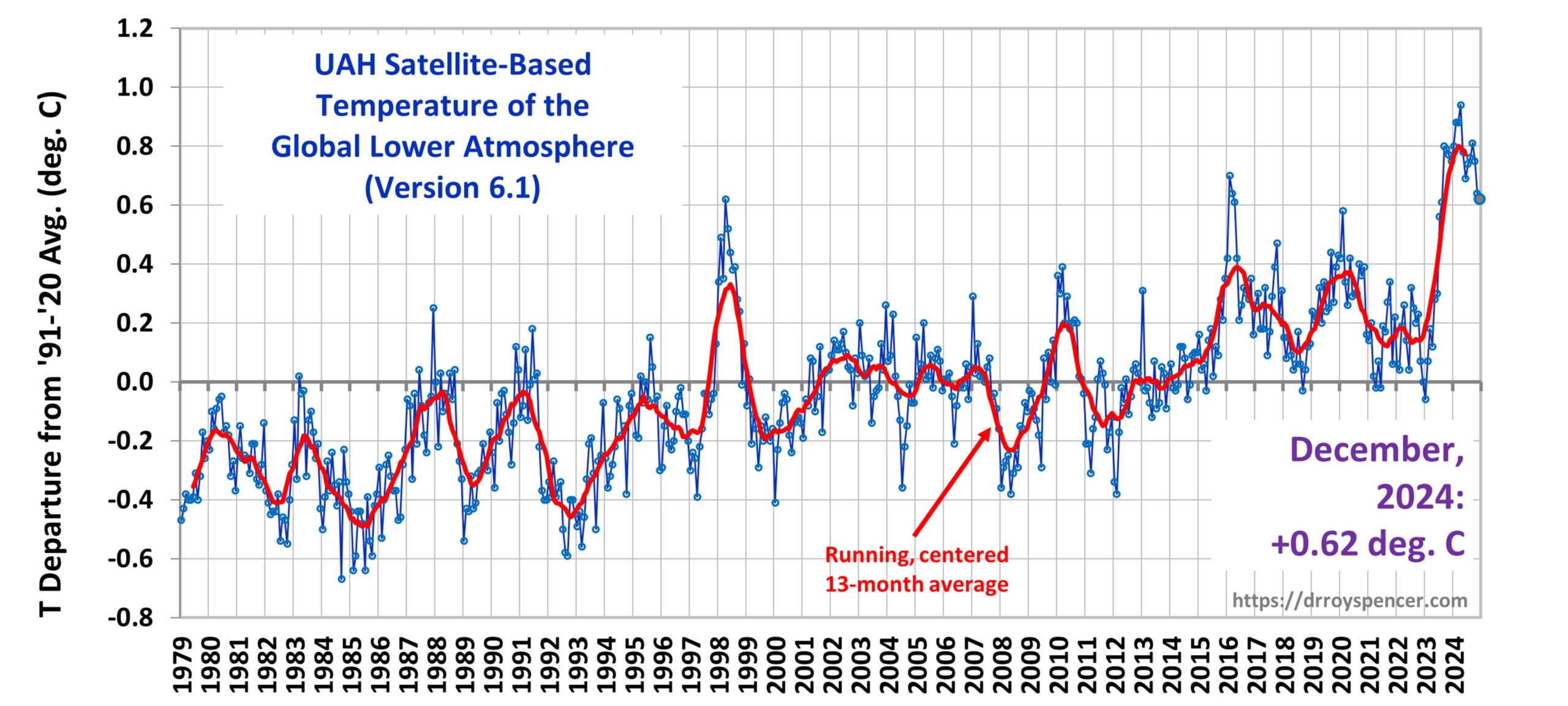
The Version 6.1 global average lower tropospheric temperature (LT) anomaly for December, 2024 was +0.62 deg. C departure from the 1991-2020 mean, down slightly from the November, 2024 anomaly of +0.64 deg.
The Version 6.1 global area-averaged temperature trend (January 1979 through December 2024) remains at +0.15 deg/ C/decade (+0.22 C/decade over land, +0.13 C/decade over oceans).
As seen in the following ranking of the years from warmest to coolest, 2024 was by far the warmest in the 46-year satellite record averaging 0.77 deg. C above the 30-year mean, while the 2nd warmest year (2023) was +0.43 deg. C above the 30-year mean. [Note: These yearly average anomalies weight the individual monthly anomalies by the number of days in each month.]
The following table lists various regional Version 6.1 LT departures from the 30-year (1991-2020) average for the last 24 months (record highs are in red).
YEAR
MO
GLOBE
NHEM.
SHEM.
TROPIC
USA48
ARCTIC
AUST
2023
Jan
-0.06
+0.07
-0.19
-0.41
+0.14
-0.10
-0.45
2023
Feb
+0.07
+0.13
+0.01
-0.13
+0.64
-0.26
+0.11
2023
Mar
+0.18
+0.22
+0.14
-0.17
-1.36
+0.15
+0.58
2023
Apr
+0.12
+0.04
+0.20
-0.09
-0.40
+0.47
+0.41
2023
May
+0.28
+0.16
+0.41
+0.32
+0.37
+0.52
+0.10
2023
June
+0.30
+0.33
+0.28
+0.51
-0.55
+0.29
+0.20
2023
July
+0.56
+0.59
+0.54
+0.83
+0.28
+0.79
+1.42
2023
Aug
+0.61
+0.77
+0.45
+0.78
+0.71
+1.49
+1.30
2023
Sep
+0.80
+0.84
+0.76
+0.82
+0.25
+1.11
+1.17
2023
Oct
+0.79
+0.85
+0.72
+0.85
+0.83
+0.81
+0.57
2023
Nov
+0.77
+0.87
+0.67
+0.87
+0.50
+1.08
+0.29
2023
Dec
+0.75
+0.92
+0.57
+1.01
+1.22
+0.31
+0.70
2024
Jan
+0.80
+1.02
+0.58
+1.20
-0.19
+0.40
+1.12
2024
Feb
+0.88
+0.95
+0.81
+1.17
+1.31
+0.86
+1.16
2024
Mar
+0.88
+0.96
+0.80
+1.26
+0.22
+1.05
+1.34
2024
Apr
+0.94
+1.12
+0.77
+1.15
+0.86
+0.88
+0.54
2024
May
+0.78
+0.77
+0.78
+1.20
+0.05
+0.22
+0.53
2024
June
+0.69
+0.78
+0.60
+0.85
+1.37
+0.64
+0.91
2024
July
+0.74
+0.86
+0.62
+0.97
+0.44
+0.56
-0.06
2024
Aug
+0.76
+0.82
+0.70
+0.75
+0.41
+0.88
+1.75
2024
Sep
+0.81
+1.04
+0.58
+0.82
+1.32
+1.48
+0.98
2024
Oct
+0.75
+0.89
+0.61
+0.64
+1.90
+0.81
+1.09
2024
Nov
+0.64
+0.88
+0.41
+0.53
+1.12
+0.79
+1.00
2024
Dec
+0.62
+0.76
+0.48
+0.53
+1.42
+1.12
+1.54
The full UAH Global Temperature Report, along with the LT global gridpoint anomaly image for December, 2024, and a more detailed analysis by John Christy, should be available within the next several days here.
The monthly anomalies for various regions for the four deep layers we monitor from satellites will be available in the next several days at the following locations:
Previous research has shown the temperatures recorded at Death Valley National Park (DVNP) have curious warm biases on very hot days, possibly due to instrument deficiencies or proximity to mounting structure apparatus and other manmade structures.
Here it is shown from 21 years of summertime (June, July, August) data that DVNP has many more days when temperatures are much higher than those at the nearby Stovepipe Wells station, than when Stovepipe Wells has hotter days than DVNP station.
These lines of evidence suggest that the hot summer daytime temperatures reported at Death Valley National Park have potentially large biases, and should only be used for their entertainment value.
In our continuing examination of the world record hottest temperature of 134 deg. F recorded at Greenland Ranch (now Death Valley National Park station) on 10 July 1913, we are finding some curious behavior in recent summertime temperatures there. (The Bulletin of the American Meteorological Society [BAMS] has accepted my proposal for a BAMS article showing the evidence that the 134 deg. F world record was 8 to 10 deg. F higher than what actually existed on that date [10 July 1913]).
Previous Work on Excessively Hot Death Valley Temperatures
Climatologist, weather observer, and storm chaser Bill Reid has blogged extensively over the years on the evidence against the 134 deg. F world record. A good place to start is his most recent post (Part 6) that deals with the Greenland Ranch foreman who made the excessively hot temperature measurements in the first half of July 1913. Bill has agreed to co-author the BAMS paper with John Christy and me.
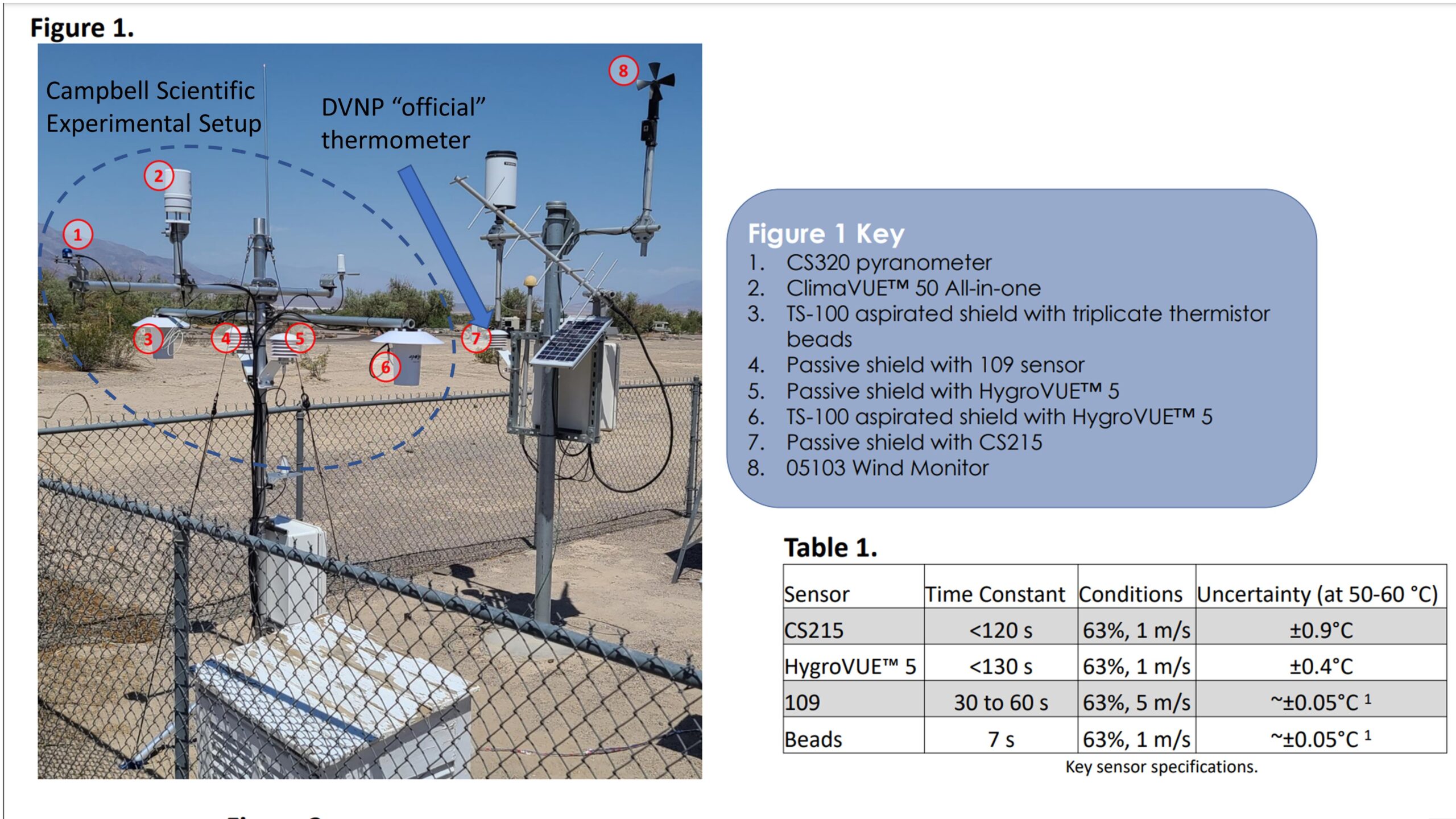
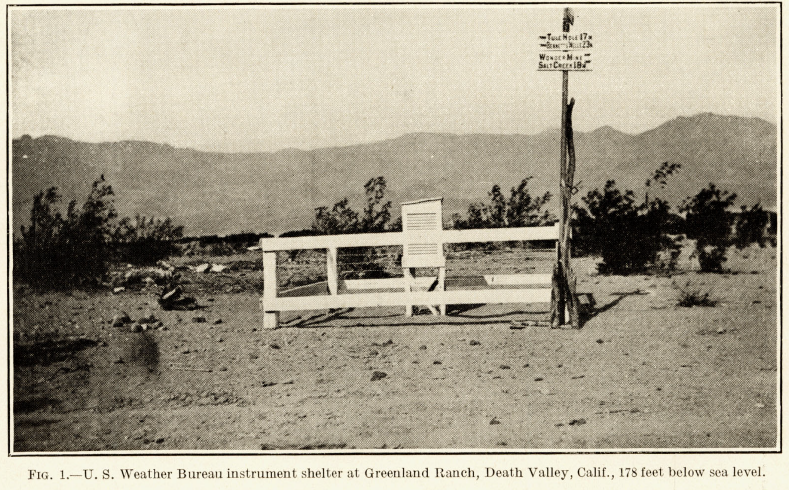
There was also an experiment carried out with a variety of temperature instrumentation placed next to the DVNP weather station during 2021 and 2022. This revealed that on the near-record hot day of 9 July 2021 (130 deg. F), the “official” DVNP sensor produced temperatures a few degrees hotter than the other instruments (AMS conference poster here). The photo in Fig. 1 shows that the older-style DVNP instrument (which is not aspirated) is mounted next to a lot of metal structure and a small solar panel.
Fig. 1 Death Valley National Park weather station, with additional instrumentation added by Dirk Baker (Campbell Scientific, Inc.) and co-investigators to compare to the ‘official’ temperature readings in 2021 and 2022. (Figure adapted from this AMS conference presentation).
The experimental setup in Fig. 1 used several temperature sensors, some with aspirated shields, others with no aspiration. The data shown in their AMS conference presentation suggests to me that the near-record 130 deg. F reading on 9 July 2021 was 2-3 deg. F too hot partly because of the non-aspirated design of the sensor. There was some additional warm bias that could have been due to all of the mounting structure seen in Fig. 1, including a small solar panel next to the DVNP station sensor.
More Evidence: DVNP vs. Stovepipe Wells Temperatures
For the last 21 years there have been two stations in Death Valley: the DVNP station next to the Furnace Creek Visitors Center, and a climate reference network (CRN) station at Stovepipe Wells, 29 km northwest of the DVNP station.
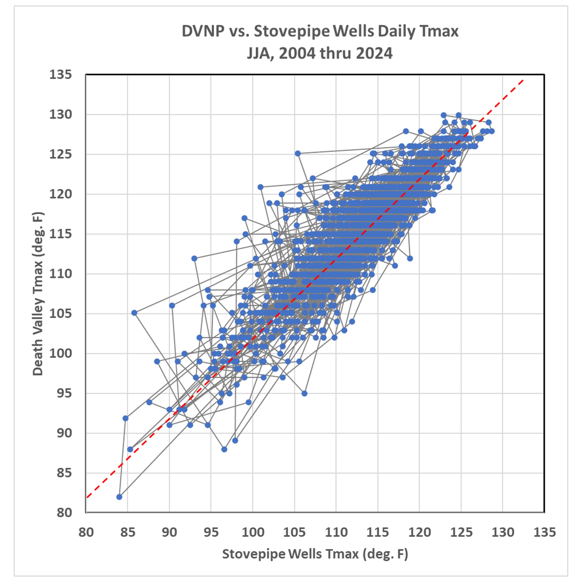
Fig. 2 shows a comparison of the daily maximum temperatures (Tmax) recorded at these two stations for every day in June, July, and August in all years from 2004 through 2024.
Fig. 2. Comparison between daily high temperatures (Tmax) recorded at Stovepipe Wells and Death Valley National Park, for all days in June, July, and August for the years 2004 through 2024. The dashed red line represents the median difference between the 2 stations (2 deg. F, DVNP warmer than Stovepipe Wells). Gray lines connect the days in chronological order.
The median of the Tmax differences between these 2 stations is 2 deg. F (DVNP warmer, represented by the dashed red line), while the average difference is 2.3 deg. F. The expected difference based upon elevation alone is 1.3 deg. F (DVNP station is 278 ft lower in elevation than Stovepipe Wells).
Note in Fig. 2 that there seem to be more outliers to the left of the dashed red line than to the right. That is, there are more days where DVNP is much warmer than Stovepipe Wells than there are days when Stovepipe Wells is much warmer than DVNP station.
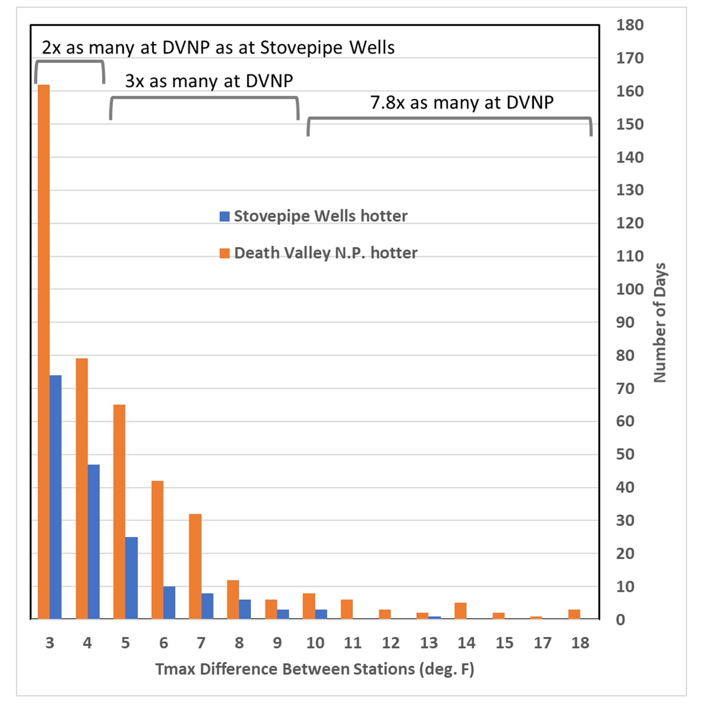
This can be better seen if we look at a frequency distribution of these station differences, adjusted for the 2 deg. F median difference between stations (Fig. 3).
Fig. 3. Frequency distributions of how many days where one Death Valley station is hotter than the other. This is after shifting of the distributions to account for a 2 deg. F difference in their median difference.
As shown in Fig. 3, DVNP station has many more days where it is hotter than Stovepipe Wells, than Stovepipe Wells has days that are hotter than DVNP station. For the 3-4 deg. F hotter category, the difference is 2X, for the 5 to 9 deg. F hotter category the difference is 3x, and for 10 deg. F or greater the difference is 7.8X.
This suggests there is something wrong with the Death Valley National Park instrumentation itself or the immediate environment around the temperature sensor that causes some days to be biased too hot. Bill Reid, who has researched this issue extensively, suspects that days with low wind have excessive heat build-up at the DVNP thermometer site, both in the general area around the instrumentation, and due to the non-aspirated design of the temperature sensor used there.
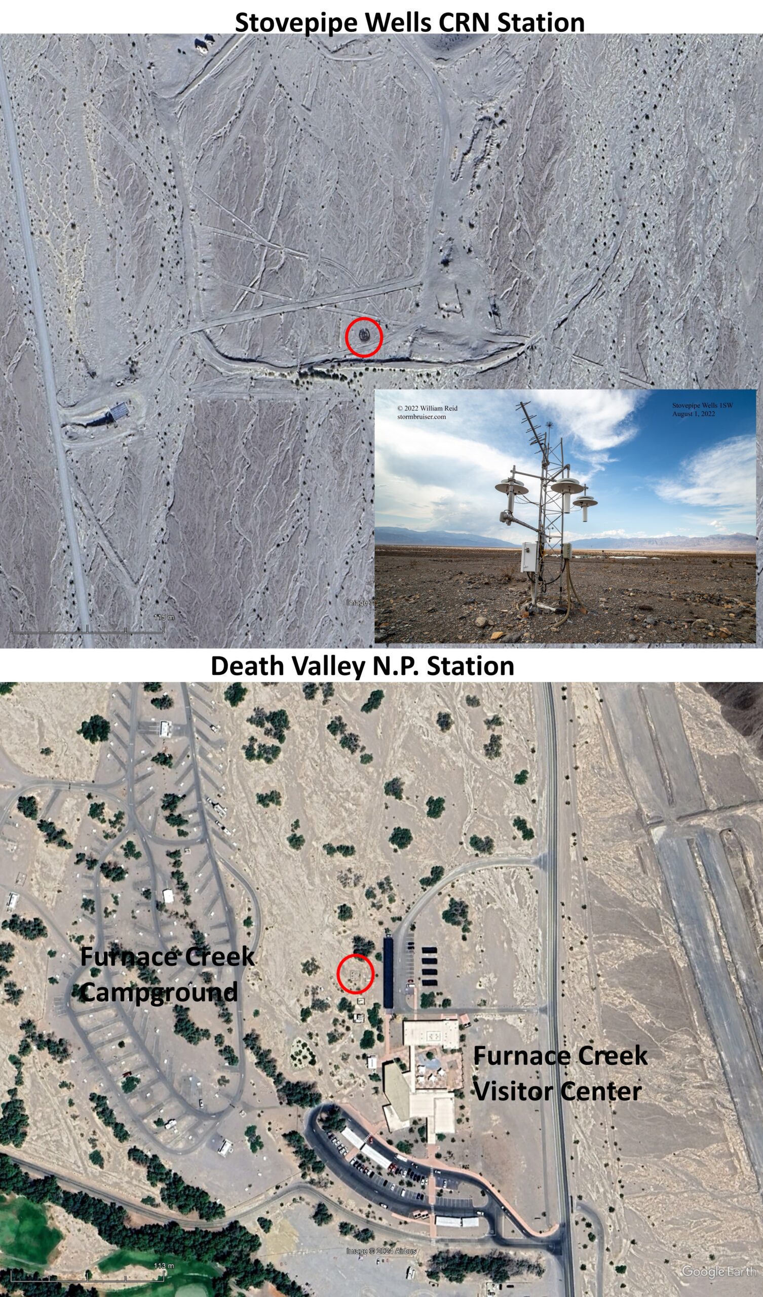
The difference in exposure at DVNP station and Stovepipe Wells is shown in Fig. 4.
Fig. 4. Google Earth imagery of Stovepipe Wells station (top) and Death Valley N.P. station (bottom), stations circled in red. The inset photo at top is of the Stovepipe Wells Climate Reference Network station, courtesy of William T. Reid. The E-W distance across these images is just over 0.5 km.
As can be seen in Fig. 4, the Death Valley N.P station has quite a bit of development surrounding the station, with parking lots, a paved campground, the Visitors Center, solar panels (black) and trees just to the south. The Stovepipe Wells site has almost no development and no vegetation. It is possible that during the prevailing southerly wind flow during the summer, the structures and trees to the south of the DVNP station lead to stagnation of air flow around the temperature sensor.
Conclusions
The evidence presented here, along with evidence presented previously by Bill Reid, Dirk Baker, and others, suggests that Death Valley National Park temperatures should not be relied upon for accurate daytime readings, and that near-record temperatures there are biased too high. The reasons for the biases are not obvious, but the evidence suggests poor sensor ventilation during the daytime when various structures in the vicinity heat up: whether the shield of the sensor itself, its supporting structure, or various manmade objects around the station site. It is also possible that the trees and other structures to the south of the station restrict air flow, further reducing effective convective heat transport away from the solar heated desert surface.
It is my opinion that “official” Death Valley temperatures should use the Stovepipe Wells site data, which come from state-of-the-art Climate Reference Network instrumentation. The traditional site near the Death Valley National Park Visitors Center should only be used for entertainment purposes.
Maybe the National Park Service should investigate adding a CRN station; a good location would be about 1.6 km southwest of the current station, well away from the Furnace Creek tourist area.
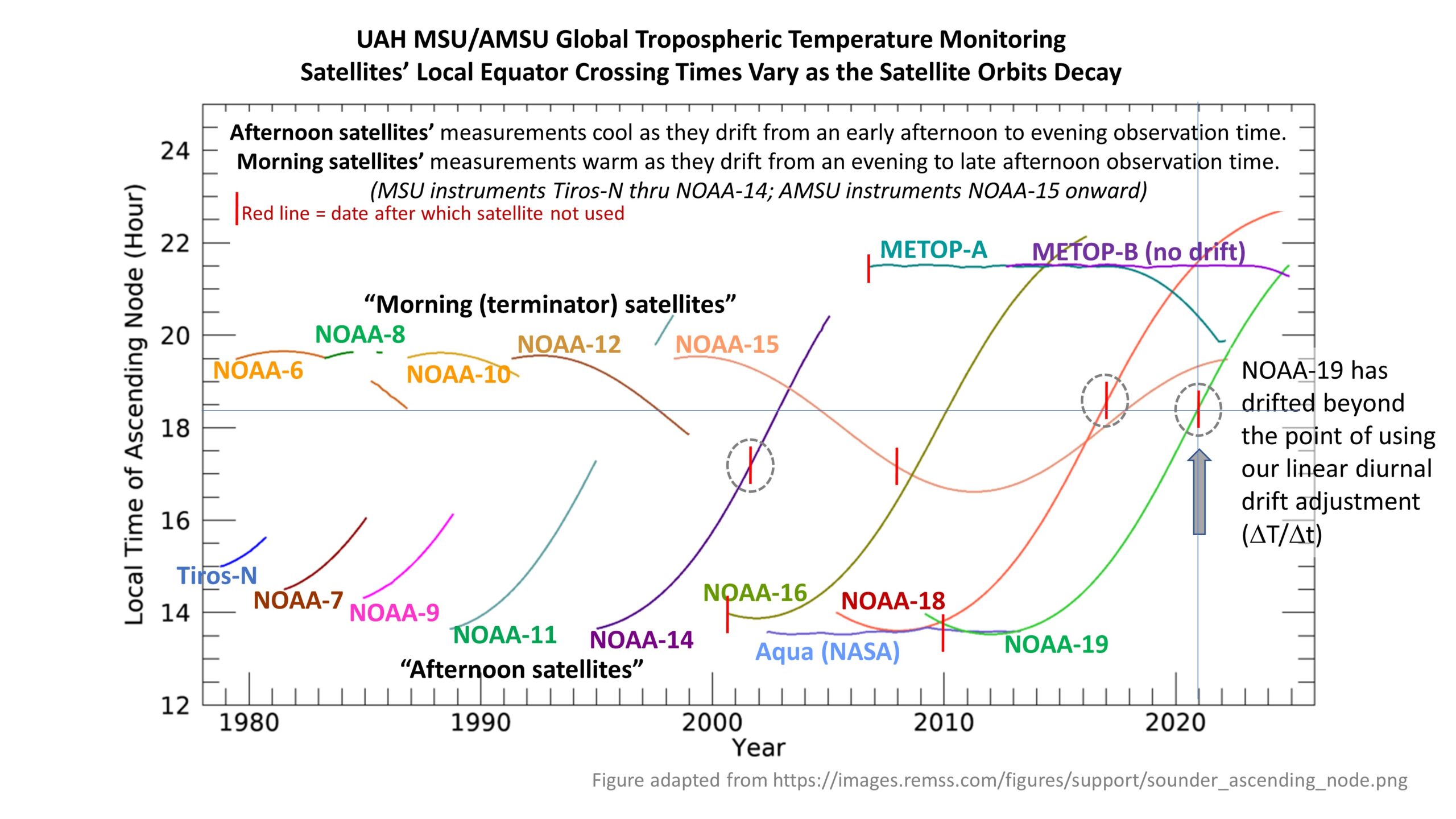
With this update, we have added Metop-C to our processing, so along with Metop-B we are back to having two satellites in the processing stream. The Metop-C data record begins in July of 2019. Like Metop-B, Metop-C was designed to use fuel to maintain its orbital altitude and inclination, so (until fuel reserves are depleted) there is no diurnal drift adjustment needed. Metop-B is beginning to show some drift in the last year or so, but it’s too little at this point to worry about any diurnal drift correction.
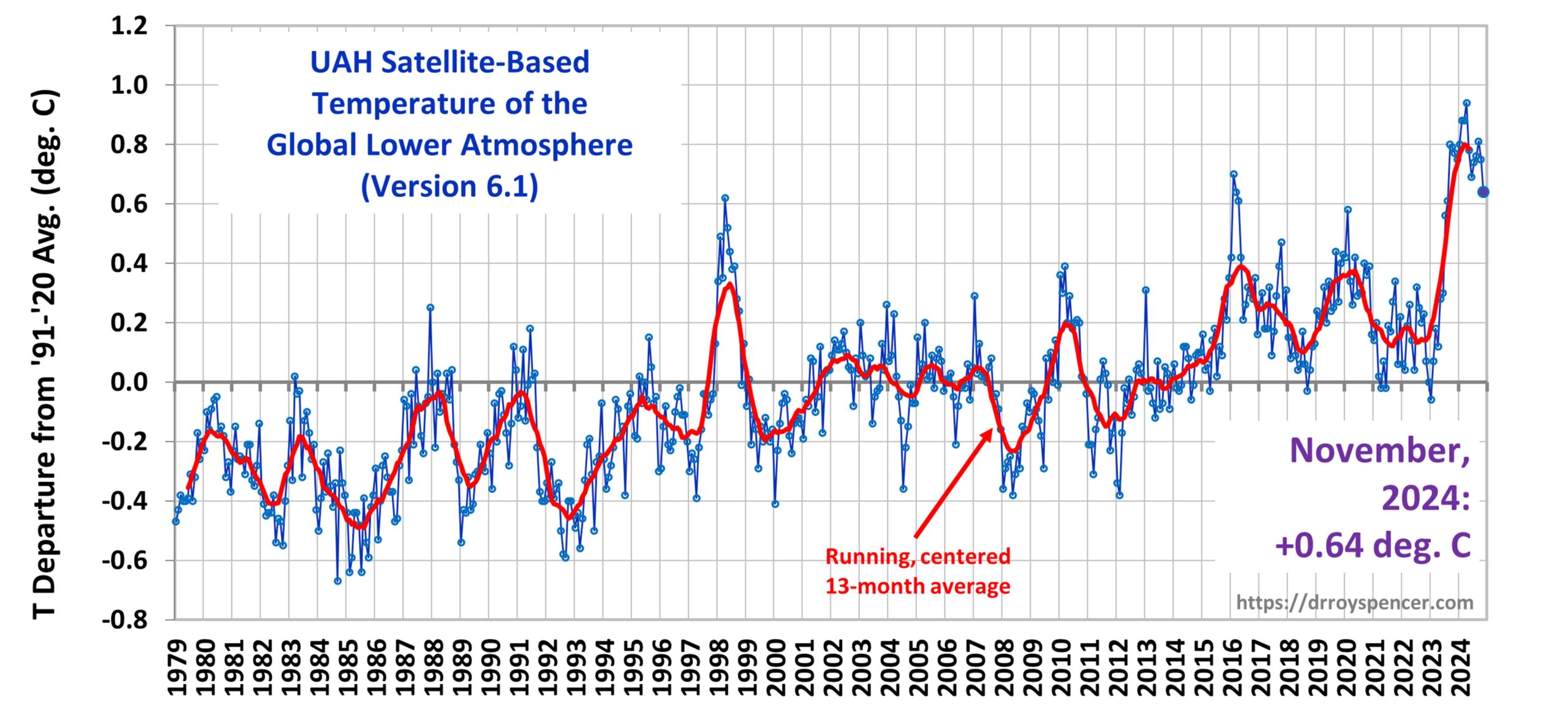
The Version 6.1 global average lower tropospheric temperature (LT) anomaly for November, 2024 was +0.64 deg. C departure from the 1991-2020 mean, down from the October, 2024 anomaly of +0.75 deg. C.
The Version 6.1 global area-averaged temperature trend (January 1979 through November 2024) remains at +0.15 deg/ C/decade (+0.21 C/decade over land, +0.13 C/decade over oceans).
The following table lists various regional Version 6.1 LT departures from the 30-year (1991-2020) average for the last 23 months (record highs are in red). Note the tropics have cooled by 0.72 deg. C in the last 8 months, consistent with the onset of La Nina conditions.
YEAR
MO
GLOBE
NHEM.
SHEM.
TROPIC
USA48
ARCTIC
AUST
2023
Jan
-0.06
+0.07
-0.19
-0.41
+0.14
-0.10
-0.45
2023
Feb
+0.07
+0.13
+0.01
-0.13
+0.64
-0.26
+0.11
2023
Mar
+0.18
+0.22
+0.14
-0.17
-1.36
+0.15
+0.58
2023
Apr
+0.12
+0.04
+0.20
-0.09
-0.40
+0.47
+0.41
2023
May
+0.28
+0.16
+0.41
+0.32
+0.37
+0.52
+0.10
2023
June
+0.30
+0.33
+0.28
+0.51
-0.55
+0.29
+0.20
2023
July
+0.56
+0.59
+0.54
+0.83
+0.28
+0.79
+1.42
2023
Aug
+0.61
+0.77
+0.45
+0.78
+0.71
+1.49
+1.30
2023
Sep
+0.80
+0.84
+0.76
+0.82
+0.25
+1.11
+1.17
2023
Oct
+0.79
+0.85
+0.72
+0.85
+0.83
+0.81
+0.57
2023
Nov
+0.77
+0.87
+0.67
+0.87
+0.50
+1.08
+0.29
2023
Dec
+0.75
+0.92
+0.57
+1.01
+1.22
+0.31
+0.70
2024
Jan
+0.80
+1.02
+0.58
+1.20
-0.19
+0.40
+1.12
2024
Feb
+0.88
+0.95
+0.81
+1.17
+1.31
+0.86
+1.16
2024
Mar
+0.88
+0.96
+0.80
+1.26
+0.22
+1.05
+1.34
2024
Apr
+0.94
+1.12
+0.77
+1.15
+0.86
+0.88
+0.54
2024
May
+0.78
+0.77
+0.78
+1.20
+0.05
+0.22
+0.53
2024
June
+0.69
+0.78
+0.60
+0.85
+1.37
+0.64
+0.91
2024
July
+0.74
+0.86
+0.62
+0.97
+0.44
+0.56
-0.06
2024
Aug
+0.76
+0.82
+0.70
+0.75
+0.41
+0.88
+1.75
2024
Sep
+0.81
+1.04
+0.58
+0.82
+1.32
+1.48
+0.98
2024
Oct
+0.75
+0.89
+0.61
+0.64
+1.90
+0.81
+1.09
2024
Nov
+0.64
+0.88
+0.41
+0.54
+1.12
+0.79
+1.00
The full UAH Global Temperature Report, along with the LT global gridpoint anomaly image for November, 2024, and a more detailed analysis by John Christy, should be available within the next several days here.
The monthly anomalies for various regions for the four deep layers we monitor from satellites will be available in the next several days at the following locations:
Update (11/12/2024): New annotated version of Fig. 1 added. Corrected who the Greenland Ranch foreman was and associated correspondence. Will fix Fig. 2 (2021/2022) problem Wednesday morning.
Update (11/13/2024): Fixed Fig. 2
In Part 1 I claimed that using stations surrounding Death Valley is a good way to “fact check” warm season high temperatures (Tmax) at the Death Valley station, using a correction for elevation since all surrounding stations are at higher (and thus cooler) elevations. In July of each year, a large tropospheric ridge of high pressure makes the air mass in this region spatially uniform in temperature (at any given pressure altitude), and daily convective heating of the troposphere leads to a fairly predictable temperature lapse rate (the rate at which temperature falls off with height). This makes it possible to estimate Death Valley daytime temperatures from surrounding (cooler) stations even though those stations are thousands of feet higher in elevation than Greenland Ranch, which was 168 ft. below sea level.
Lapse Rates Computed from Stations Surrounding Death Valley
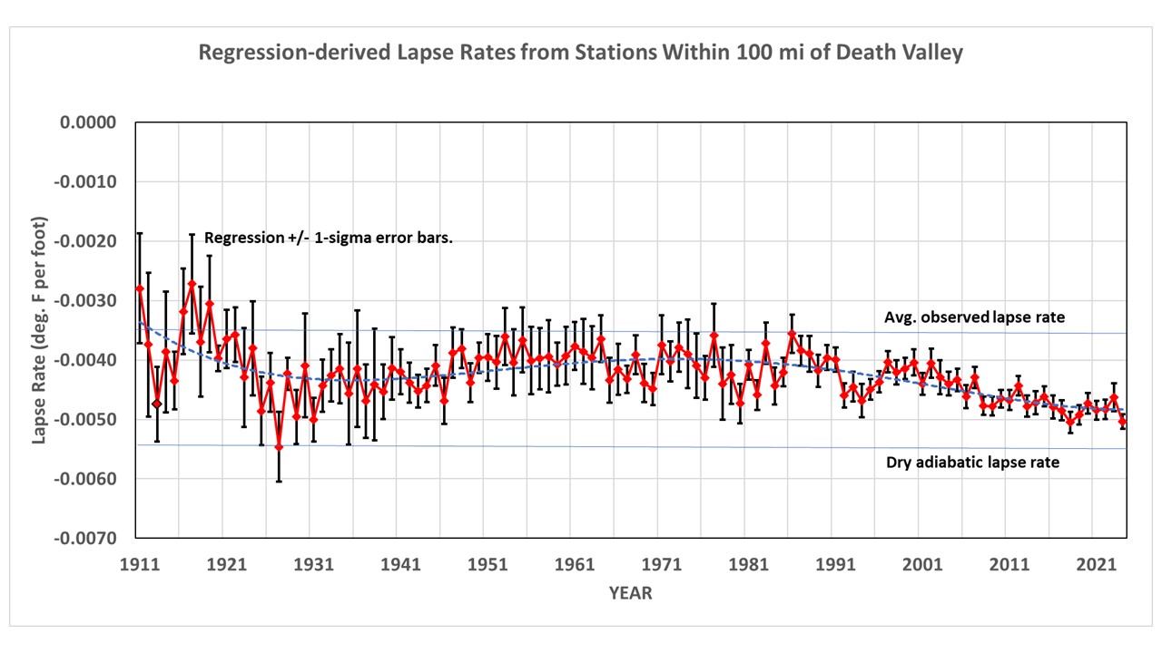
If I use all available GHCN daily stations within 100 miles of Greenland Ranch (aka Furnace Creek, aka Death Valley N.P.) in each July from 1911 to 2024 to compute the month-average lapse rate (excluding the Death Valley stations[s]), I get the results in Fig. 1.
Fig. 1. Lower tropospheric temperature lapse rate estimated from all stations within 100 miles of Greenland Ranch, Death Valley, CA. The number of available stations for these calculations range from several in the early years to 25 or more in the later years. Here I will assume a constant lapse rate of -0.004 during the 20th Century. The 4th order polynomial fit to the data would be another way to assume how the lapse rate changes over time.
The computed lapse rates mostly fall between the dry adiabatic value and the U.S. standard atmosphere value (except in the early years). Given the few stations available in the early years, I will base the calculations that follow on an assumed lapse rate of -0.004 deg F per ft. for the first half of the record, and will assume that the observed steepening of the lapse rate after the 1980s is real, with a value of -0.0048 deg. F per ft. in the early 2020s. In Part 1, I used the actual values in Fig. 1 in each year to estimate Death Valley temperatures. This time I’m using average lapse rate values over many years, keeping in mind the early decades had few stations and so their values in Fig. 1 are more uncertain.
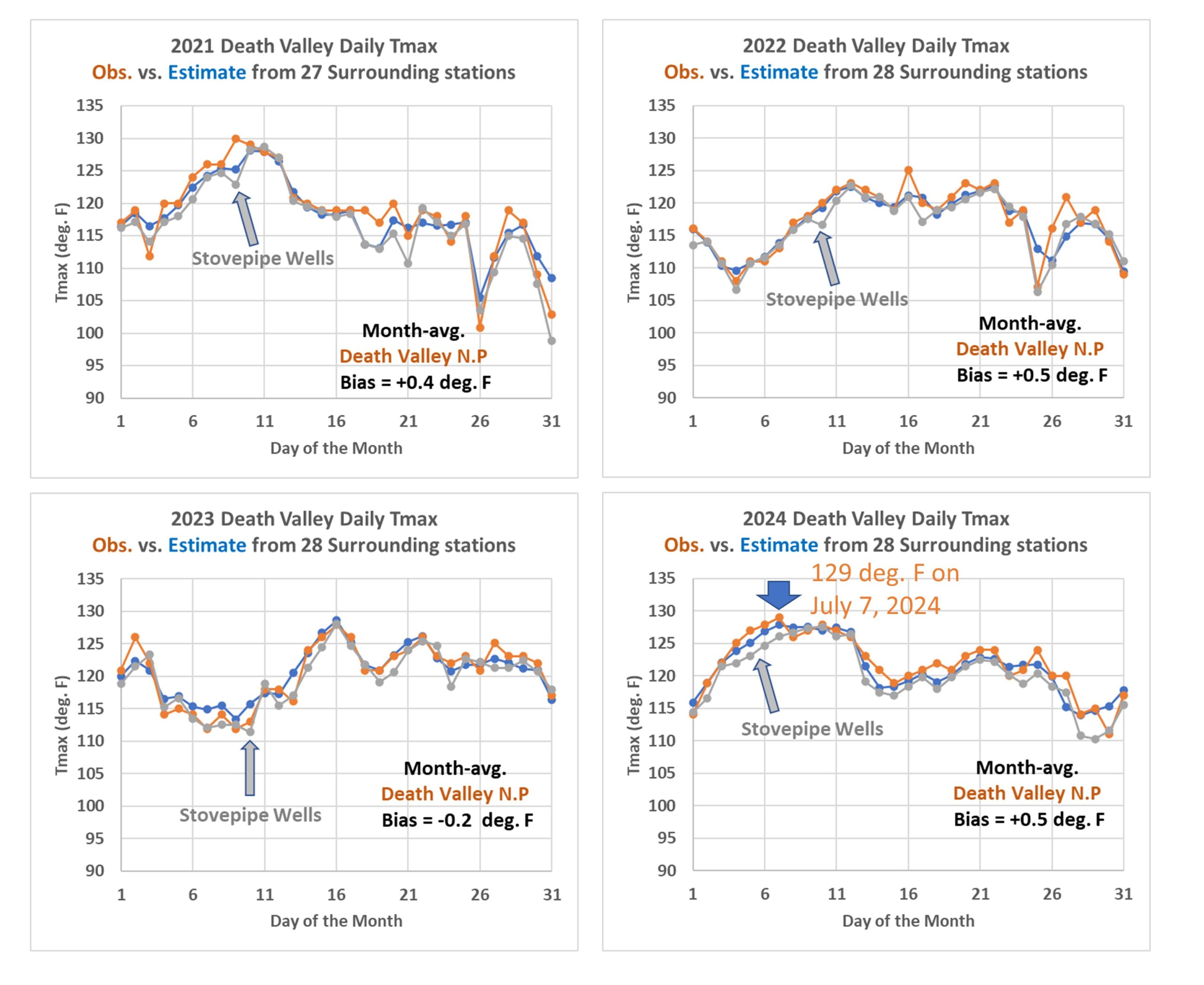
Daily Estimated July Tmax at Death Valley: 2021-2024
How accurately can we estimate daily Tmax temperatures in Death Valley from surrounding high-elevation stations? The following plot (Fig. 2) shows how the July daily observed Tmax temperatures in Death Valley (2021, 2022, 2023, 2024, orange for Death Valley N.P.) compare to estimates made based upon surrounding, high-elevations stations (blue), assuming a lapse rate of -0.0048 deg. F per ft (see Fig. 1).
Fig. 2. Daily estimated July Tmax temperatures for Death Valley N.P. from surrounding stations (blue) compared to those observed (orange, 194 ft. below sea level)for 2021, 2022, 2023 and 2024.
In each year the daily estimates from surrounding stations (blue) are reasonably close (within a couple of degrees) to the observed values at both Death Valley N. P. (orange) and at the nearby station Stovepipe Wells. For example, on July 7, 2024 the observed “near record” value of 129 deg. F degrees agrees well with the lapse-rate estimated value of 128 deg. F. Note there were many (27 of 28) stations within 100 miles of Death Valley available to make these estimates during these years.
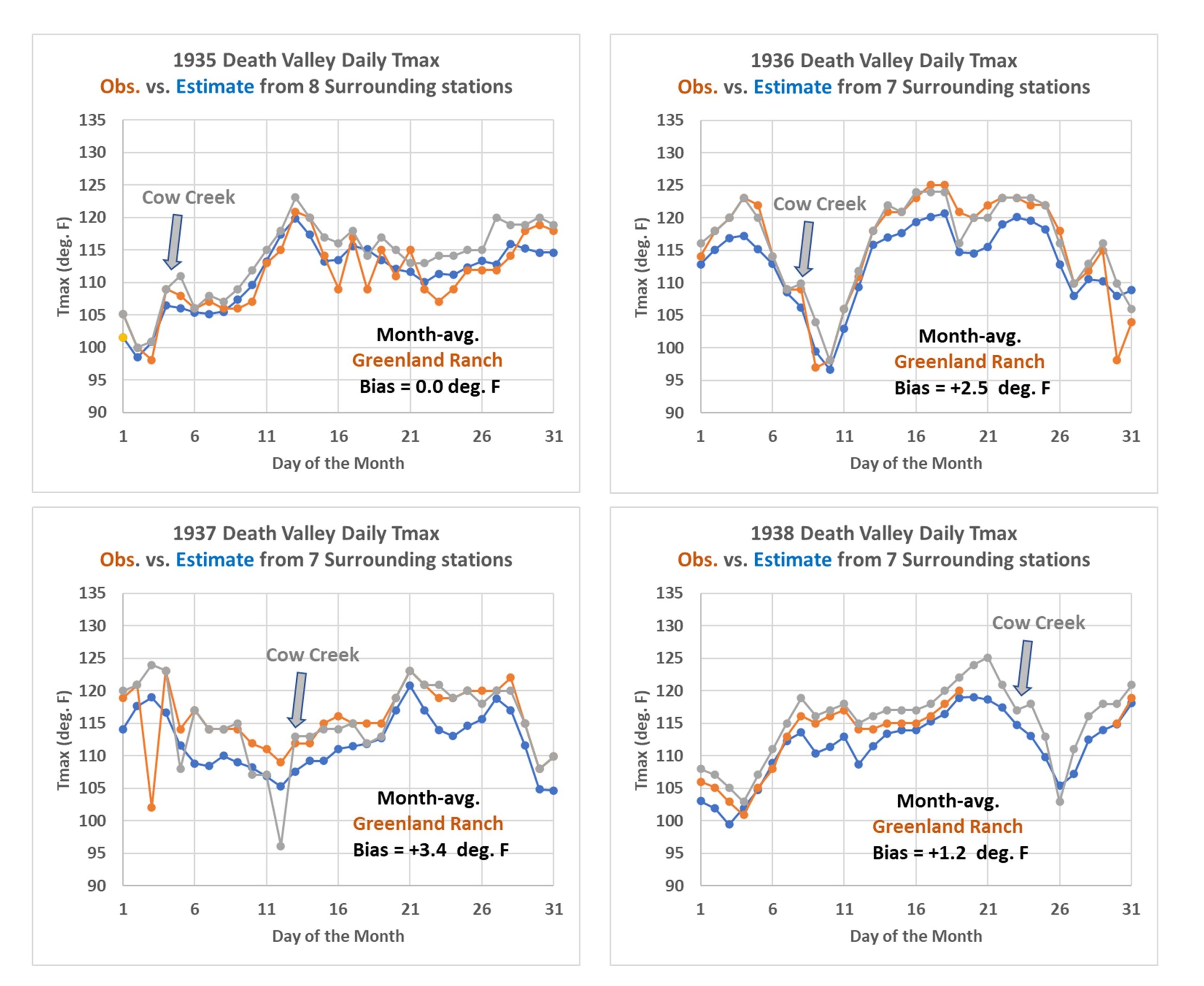
Daily Estimated July Tmax at Death Valley: 1935-1938
Next, let’s travel back to the 1930s, when there were fewer stations to do these estimates (Fig. 3).
Fig. 3. Daily estimated Tmax temperatures for Death Valley during 1935, 1936, 1937, 1938 from surrounding stations (blue) compared to those observed at Greenland Ranch (orange, 168 ft. below sea level) and Cow Creek (grey, 151 t. below sea level).
Despite only having 7 or 8 stations from which to estimate Death Valley temperatures, the agreement is still reasonably good in 1935, with no bias between observed and estimated, but 1-3 deg. F bias at Greenland Ranch vs. estimated in the following 3 years. There are also a few low temperature outliers in 1937-38 at Greenland Ranch and Cow Creek; I don’t know the reason for these.
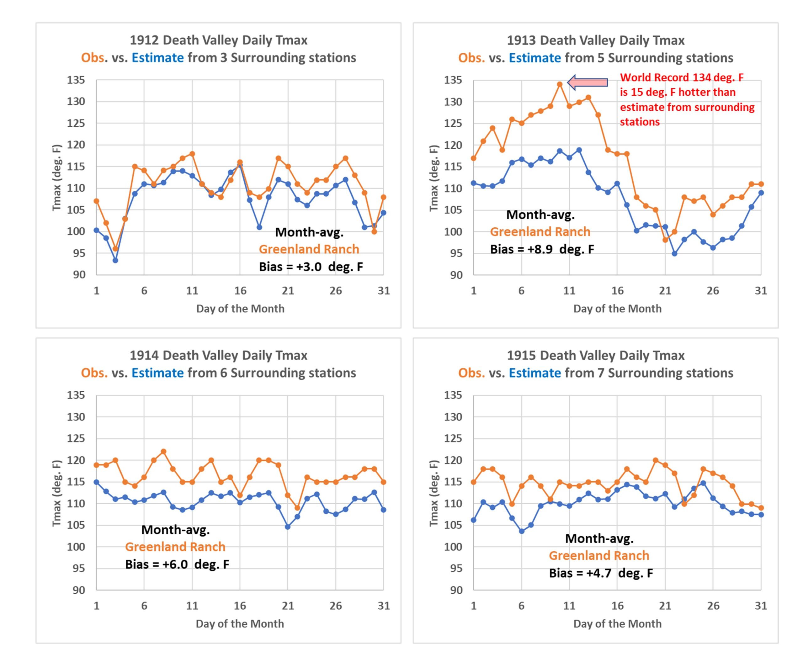
Daily Estimated July Tmax at Death Valley: 1912-1915
Finally we examine the period in question, when the 134 deg. F world record temperature was recorded on July 10, 1913 (Fig. 4).
Fig. 4. Daily estimated Tmax temperatures for Death Valley during 1912, 1913, 1914, 1915 from surrounding stations (blue) compared to those observed at Greenland Ranch (orange, 168 ft. below sea level).
During these years there were only 3 to 7 stations from which to compute Death Valley Tmax. In 1912, despite only 3 stations, the reported temperatures averaged only 3 deg. F above those estimated from surrounding stations. But in 1913 (the year of the record) the observations averaged an astounding 9 deg. F warmer than the surrounding 5 stations would have suggested. On July 10, the excess was 15 deg. F!
That second week of July 1913 was indeed unusually hot, and it was during this time that the ranch foreman (Oscar Denton) responsible for making the temperature readings from an official instrument shelter provided by the U.S. Weather Bureau in 1911 might have replaced the official values with values that more accorded with the heat he and his supervisor (Fred Corkill) were feeling on his veranda, away from the USWB instrument shelter which was sited next to an irrigated field. Bill Reid covers the details of correspondence between Corkill and a USWB official in San Francisco regarding the shelter temperatures and how much cooler they were compared to what was measured by a second thermometer farther away from the irrigated field. Reid believes (and I agree) that the shelter temperatures were, at least for a time while Denton was responsible for tabulating the daily measurements, replaced with measurements from a separate thermometer having uncertain quality and siting away from hot surfaces exposed to the sun.
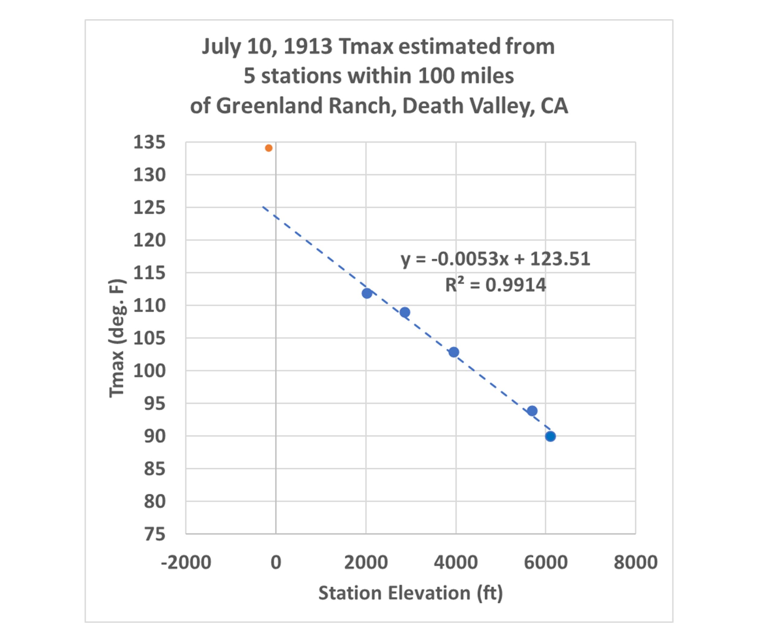
So, How Much Hot Bias Exists in the 134 deg. F “World Record”?
We will never know exactly how much warm bias exists in the world record value. But from comparison to the biases in 1912 and 1914, I would say 9 to 12 deg. F is a reasonable estimate.
Of course, this might be adjusted somewhat if one assumes a slightly different lapse rate than the -0.004 deg. F per ft. I have assumed here (see Fig. 1). For instance, what if the air mass on July 10, 1913 had an exceptionally steep lapse rate, such that an even greater adjustment for elevation needed to be made to estimate the hot temperature in Death Valley? If I use use the lapse rate estimated from the 5 surrounding stations on July 10, 1913 (see Fig. 5), that lapse rate value is indeed “steeper”, at -0.0053 deg. F per ft. But if we use that value to estimate the Death Valley temperature, it is still 10 deg. cooler than the 134 deg. F recorded value. This is still within the 9 to 12 degree bias range I mentioned above.
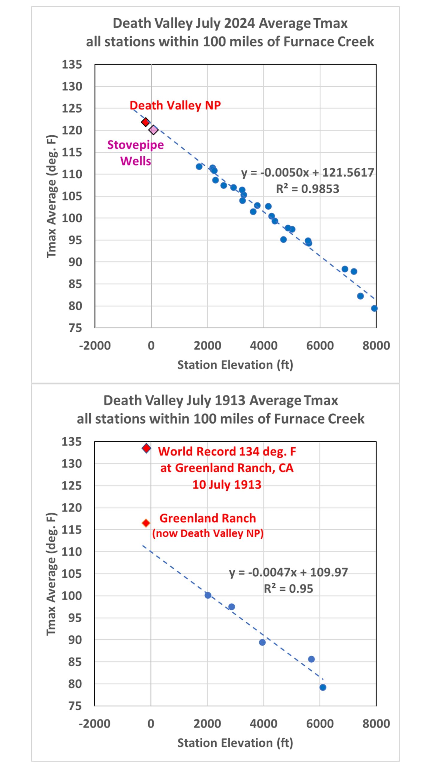
Fig. 5. The world record value of 134 deg. F (red) is 10 deg. F warmer than that suggested by the surrounding higher-elevations stations’ temperature variations with elevationon July 10, 1913.
Conclusion
The 134 deg. F world record hottest temperature from Death Valley is likely around 10 deg. F too high, compared to elevation-adjusted temperatures from surrounding stations. The most likely cause is that the ranch foreman’s reported measurements were (shall we say) unacademically recorded. I find it rather remarkable that the world record hottest temperature from Death Valley was not revised many years ago, since the methods for “fact checking” the record are fairly simple, and based upon meteorological principles known for well over 50 years.
NOTE:Since he has done extensive investigation into some implausibly hot temperatures reported in Death Valley, I asked Bill Reid to comment on my previous blog post where I maintain that the world record 134 deg. F highest recorded air temperature was likely biased warm by about 10 deg., and should not be accepted as a world record. What follows are Bill’s initial thoughts on the subject. Also, based upon his comments, I will likely update the charts found in my previous blog post with more realistic temperature lapse rate values in the early 20th Century when insufficient stations were available to determine accurate lapse rates.
by William T. Reid
A big thank you to Dr. Spencer for investigating the current (very dubious) world high-temperature record and for bringing attention to my Death Valley climate research. There are a handful of ways, both climatologically and meteorologically, to show that Greenland Ranch’s reported maximum of 134F on July 10, 1913, is likely not valid.
Dr. Spencer’s methodology here (comparing the Death Valley maximums to those the closest surrounding stations, with adjustments for station elevation) is indeed a devastating blow to the authenticity of the suspect observations. What it basically demonstrates is that the lower troposphere was not hot enough to support temperatures much above 125F in July, 1913. I have compared regional maximums for all of the hottest summertime events since 1911. In practically all instances (in which the Greenland Ranch and Death Valley reports appear reasonable), ALL of the maximums at the closest surrounding stations lend support to the maximums for Death Valley.
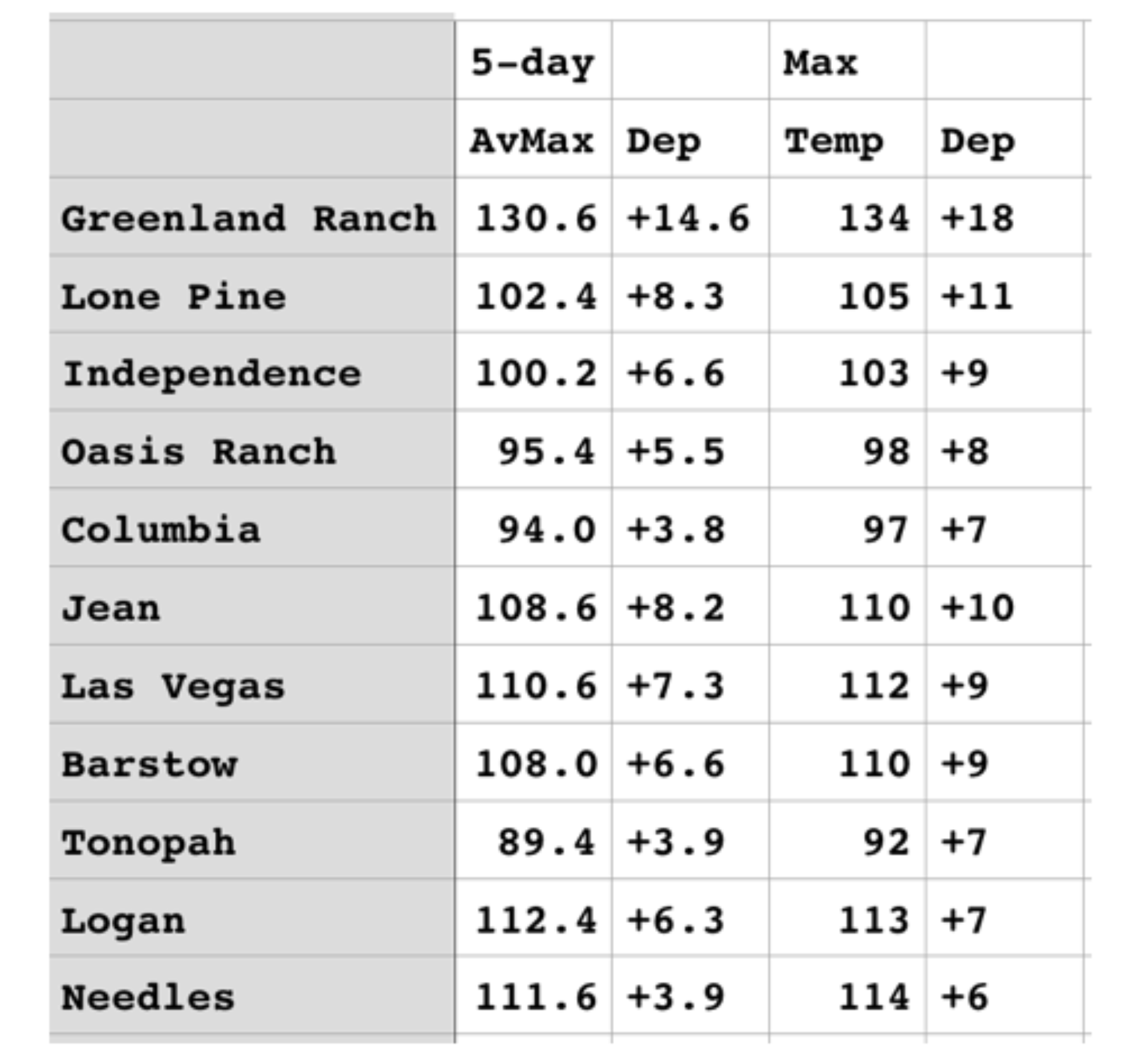
From July 7 to 14 of 1913, when eight consecutive afternoons had reported maximums of 127, 128, 129, 134, 129, 130, 131 and 127F in Death Valley, NONE of the maximums from the closest surrounding stations supported the Greenland Ranch maximums! The departures from average for maximums for the hottest five-day stretch were about +4 to +8 at the closest stations, while maximums at Greenland Ranch were nearly 15 degrees F above the average for July. (see table)
Annual maximums at Greenland Ranch from 1911 to 1960 ranged from 120F to 127F, except for the 134F in 1913. If the reported maximums at Greenland Ranch in July, 1913, were authentic, then the maximums at the closest surrounding stations in that month would have been much higher than reported. In addition, numerous regional heat waves have been hotter than the one during the first half of July, 1913. Why have Death Valley maximums failed to exceed 130F in the interim when three days in July 1913 purportedly reached 134, 130 and 131F?
In his “bias” chart, Dr. Spencer notes the “substantial warm biases in the temperatures reported at Greenland Ranch in the first 10-15 years.” And, he mentions that the observer(s) may have been relying to some extent on thermometers other than the official instrumentation. I do think that the observer was comparing “household thermometer” readings with the official equipment on occasion from spring to summer of 1913. Higher readings off of the poorly-exposed thermometers near the ranch house and under the veranda were probably (and inappropriately) entered onto the official climate form. But, I have not uncovered much evidence of this particular type of deviation from standard observational procedures outside of 1913.
I would contend that the generally higher “bias” numbers from the early years comparably are due primarily to changes at the closest area weather stations which promoted cooler maximums early on and warmer maximums later. For example, two of the closest stations to Greenland Ranch in 1913 were Independence and Lone Pine, in Owens Valley. In 1913, Owens River water was diverted to Los Angeles, and the Owens Valley gradually dried up. Summer maximums increased as Owens Lake evaporated, irrigation was not possible and farmland was abandoned, and desert-like conditions developed. (Roy’s note: The early years had very few stations within 100 miles of Death Valley, and the temperature lapse rates I computed from those few stations appear to be biased as a result. I will correct this in a future blog post, and will provide what should be better estimates of average July daily maximum Death Valley temperatures.)
Also, in the early decades of the 20th century, thermometer shelters were (almost invariably) sited above grass. This resulted in very conservative (i.e., coolish) maximums at desert stations. Low humidities promoted cooling due to evapotranspiration effects. In the early decades of the 20th century, desert weather stations were generally in towns, amidst shade trees and lawns. The resulting maximum temperature reports were very conservative. By mid-century and thereafter, the town weather stations were more likely to be at the airport or at a municipal utility site, fire station or equipment yard. Grass cover and shade trees were usually absent at these locales. Today, desert weather stations in towns and cities are (almost invariably!) above bare ground.
You can imagine the difference in maximums between desert stations above oft-irrigated grass and those above bare ground. (Roy’s note: In my experience, unless the vegetation area is rather large, and there is almost no wind, a weather station’s daily maximum temperature will still be largely determined by air flowing from the larger-scale desert surroundings. But note… this is different from, say a poorly sited thermometer next to a brick wall or heat pump where hot air from an isolated source can elevate the daily maximum temperature recorded).
The Greenland Ranch station was originally sited above a patch of alfalfa grass, immediately adjacent to forty acres of cultivated and irrigated land.
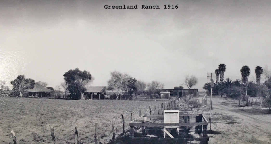
It is my belief that the new observer in 1913 (Oscar Denton) was rather disillusioned with the conservative maximums from the official station above grass and next to the evaporatively-cooled farmland. I think he felt compelled to fudge the maximums upwards in 1913. Photographs of the Greenland Ranch weather station show that it was above bare ground by about 1920 (see example photo at top of post).
Over the years, a few commentators have have argued that the world record highest temperature of 134 deg. F at Death Valley, CA recorded on July 10, 1913 is physically implausible.
Here I show quantitatively that the 134 deg F temperature is biased high, by about 10 deg. F.
Extensive historical research by William T . Reid has suggested the person making the temperature observations at Greenland Ranch likely replaced the official measurements from a thermometer in a Stevenson screen shelter with other measurements made next to the adobe living quarters.
Update #1 (11/8/2024): Fixed a few typos.
Update #2 (11/8/2024): For those messaging me about Furnace Creek temperatures reaching 130 deg. F in recent years, see Bill Reid’s summary of side-by-side measurements made there [and reported at an AMS meeting] showing the non-aspirated “official” equipment produces temperatures 2-3 deg. too high during light wind conditions.
Update #3 (11/9/2024): Bill Reid corrected my use of the term “mountain” stations to describe those not in Death Valley. Many of those stations are at desert plateau sites, so I have changed the term to “higher elevation” stations. I have also asked Bill to provide additional thoughts on this issue, which will be the next blog post here.
Background
The “official” world record highest near-surface air temperature is 134 deg. F, recorded in Death Valley, California on July, 10, 1913 at Greenland Ranch, California an isolated location with no similarly sited stations with which to compare (say, within 10 miles and below sea level). Greenland Ranch was a manmade oasis created by the Borax people around the turn of the 20th Century, with water piped in from a nearby mountain. It has a rich history, but always against a backdrop of oppressive summer heat that few visitors (and even workers) could endure.
As part of my new analyses of GHCN daily high and low temperatures, John Christy suggested I take a look at the Death Valley temperature data, and the record 134 deg. temperature in particular. Several people over the years have expressed concerns that the 134 deg. reading is implausibly high, but this has been difficult to prove. Both the World Meteorological Organization and NOAA’s National Weather Service continue to recognize 134 deg. F as the world record. It is quite likely that Death Valley remains the hottest location in North America; it’s the world record value that is in question here.
The most extensive meteorological and historical arguments against the record I’m aware of come from a series of blog posts by storm chaser, climatologist, and weather observer William T. Reid, re-posted at Weather Underground here, which I did not read until after I did the calculations which follow. I have since read some of what Bill has written, and I encourage anyone with an interest in history to read his extensive summaries (along with old photos) of Greenland Ranch, where the world record temperature was recorded. He has done considerable library research and he found a letter from the ranch foreman who expressed disappointment that the measurements from the instrumented shelter provided by the U.S. Weather Bureau in 1911 were so much lower than what he measured under his veranda. Bill suspects (and I agree) that the reported values for some period of time might well have not been from the instrumented shelter.
The method I will use to demonstrate the near-certainty of a high bias was also included in a limited fashion in Reid’s blog post (which contains a variety of meteorological arguments). I will apply the method to all years since 1911, and will show that the 134 deg. F record was approximately 10 deg. higher than what it should have been. The analyses I present are based upon the NOAA GHCN daily temperatures, with basic NOAA quality control procedures applied, thus they are from an “official” source. The GHCN dataset includes the 134 deg. F record high temperature from Death Valley.
How Can One Quality-Check the World Record Highest Temperature?
The main reason that the world record hottest temperature cannot be easily “fact-checked” is that there were no other weather stations in Death Valley at the time, and the low elevation (below sea level) of Greenland Ranch is routinely tens of degrees F hotter than at the mountain stations, which are tens of miles away and thousands of feet higher.
Yet, from a meteorological standpoint, Death Valley in the summer is the perfect place to quality check those hot temperatures from more distant, higher-elevations stations. Before I explain the reasons why, let’s first look at how Death Valley air temperatures compare to higher-elevation stations during July of this year (2024, which had near-record high temperatures), as well as during July of 1913. Following is a plot (Fig. 1) of July-average high temperatures (Tmax) for all stations within 100 miles of the Furnace Creek station (previously “Greenland Ranch”, and today called Death Valley National Park [NP] station). Importantly, I’m plotting these average temperatures versus station elevation:
Fig. 1. July average maximum temperatures at stations within 100 miles of Furnace Creek, CA in 2024 (top) and 1913 (bottom), plotted against station elevation. The regression lines are fit to all stations except those near Greenland Ranch/Furnace Creek/Death Valley N.P.
Note the strong relationship between station elevation and temperature in the 2024 data (top), something William Reid also noted. Significantly, the two lowest-elevation stations (in Death Valley) in 2024 have temperatures which are very close to the regression line that relates how the July-average high temperatures vary with station altitude (the two Death Valley stations, located below sea level, are not included in the regression). But in 1913 (bottom plot), the Greenland Ranch value departs substantially from what would be expected from the surrounding stations.
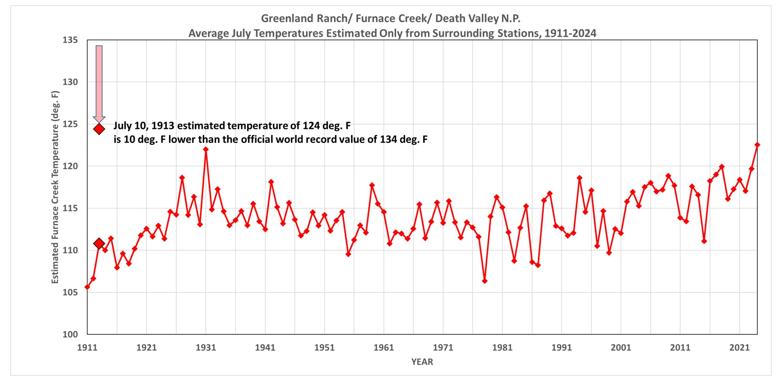
Regression lines like those in Fig. 1 can be computed in the other years, too, and used to statistically estimate what temperature the Furnace Creek station in Death Valley should have measured, based upon the surrounding, higher-altitude stations. This method allows us to estimate the Death Valley temperatures in each year, which is shown next in Fig. 2. (Bill Reid correctly points out that in the plots which follow, the results in the early years are from very few stations, and I agree that I should probably have used regression-derived lapse rates averaged from other years with more stations.)
Fig. 2. Yearly estimates of July average temperature at Furnace Creek, CA based upon all available GHCN stations within 100 miles of Furnace Creek. Each yearly estimate is based upon the station data from that year. The indicated estimate on July 10, 1913 (the date of the world record 134 deg. F reported reading) is 10 degrees cooler than the world record, at 124 deg. F. This 1-day estimate is based upon the surrounding stations only on that date. Note the 2024 value is about 0.5 deg. F above the value in 1931. Note that urban heat island effects (not accounted for here) might have biased the later half of the record to the warm side.
Meteorological Justification for the Methodology
There are solid meteorological reasons why one can use fairly distant, higher-elevation stations to check Death Valley temperatures in July. (Remember, my formal training is as a meteorologist… I only work in climate because it pays better. I actually took some of the temperature measurements contained in the GHCN daily dataset during summers in the late 1970s when I interned at the National Weather Service Office in Sault Ste. Marie, Michigan).
In simple terms, daytime temperatures during the warm season in dry, semi-desert or desert climates vary with altitude in a predictable and repeatable manner, and with little change over substantial distances. Evidence of this is shown in Fig. 1. This is much less true during the cool season, at night, or during cloudy (or even rainy) weather. This makes Death Valley in July one of the best places on Earth for fact-checking of very warm daytime temperature values. This applies very well to the southwestern U.S. in the summer (at least before monsoon rains arrive), where a semi-permanent high pressure ridge in May-July gets set up every year, with slowly subsiding (sinking) air producing mostly clear skies. This kind of weather feature has a large and uniform regional extent (unlike low pressure troughs, which can be sharp with strong horizontal temperature changes). This is related to something called the “Rossby radius of deformation“.
In simple terms, the warm, high pressure airmasses that settle in over the SW U.S. in July are spatially uniform, with strong daytime vertical mixing producing temperature lapse rates approaching the dry adiabatic value. This allows comparisons between temperature at stations up to (for example) 100 miles away. The big differences in temperatures between neighboring stations, then, are primarily due to altitude. Daytime temperatures in the summer in dry climates decrease rapidly with height (see Fig. 1), providing perfect meteorological conditions for doing the kind of comparison I’m describing here.
Estimated July Biases in the Greenland Ranch/Furnace Creek/Death Valley N.P.
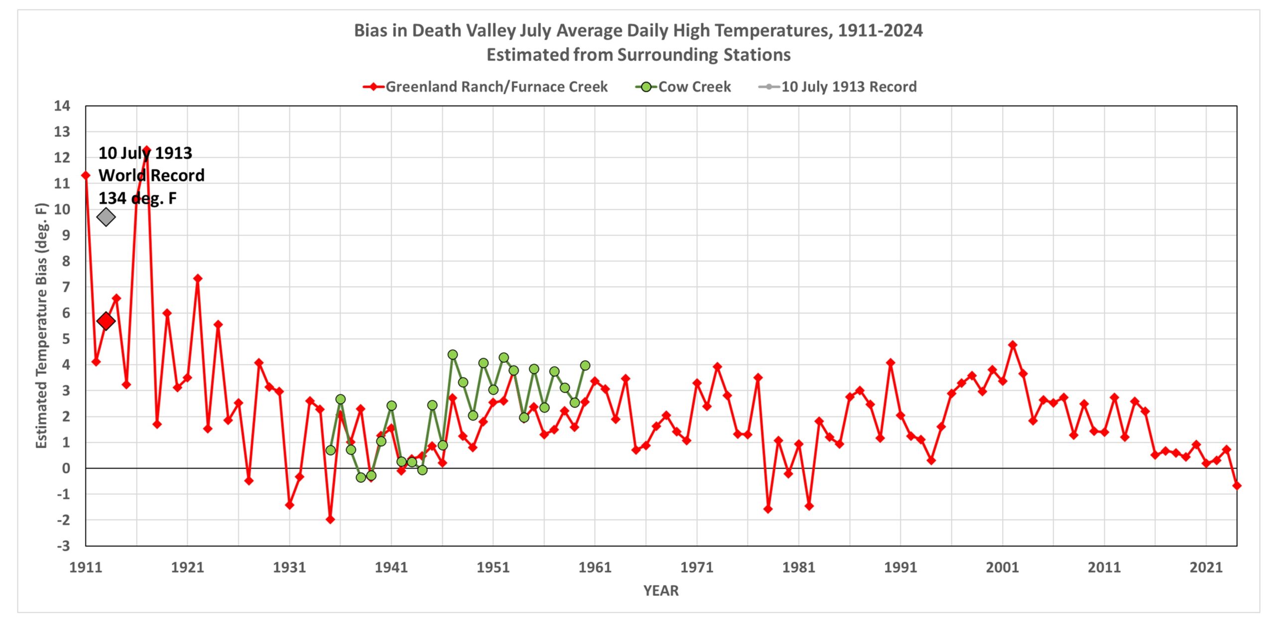
Finally, we can examine the difference between the reported July average temperatures in Death Valley from the GHCN data and the estimates from the surrounding stations (Fig. 3).
Fig. 3. Estimated biases in the official GHCN July-average temperatures in Death Valley, CA based upon comparison to Death Valley estimates made from all stations within 100 miles of Furnace Creek. The 1-2 deg. F average bias over most of the record might well not be an actual bias in the official measurements, but instead a bias in the method described. UPDATE: I will be updating Figs. 2 and 3 in a future blog post; I need to use more realistic lapse rate values in the early 20th Century when there were few stations with which to compute the lapse rate.
Note the substantial warm biases in the temperatures reported at Greenland Ranch in the first 10-15 years after the USWB installed the instrumented shelter. Again, as Bill Reid surmises, the ranch foreman was likely reporting values from a different thermometer that had poor exposure, next to a building. Also shown in green are data from a nearby station (5 miles away, at essentially the same elevation) called Cow Creek. Note that in the most recent decade, the Death Valley temperature estimates from surrounding stations agree with those measured at the current Death Valley N.P. observation site.
[I have not looked at how increasing urban heat island effects would change the details in Fig. 1-3. To the extent that urbanization has made the higher elevation stations warmer with time (I doubt urbanization is an issue at Furnace Creek), the method-estimated estimates will be correspondingly too warm, which will then cause a spurious upward trend in Fig. 2 and would reduce the computed biases seen in Fig. 3 over time, which is what we see.]
Conclusion
The bottom line is that I believe there to be sufficient quantitative evidence to say that the 134 deg. F world record hottest temperature, still recognized by the WMO and NWS, is as much as 10 deg. F too warm, likely due to observer error (which might well have been intentional). Again, for those interested in the history of Greenland Ranch (which includes the stories of those who died trying to escape the oppressive summer heat), read the fascinating history uncovered by Bill Reid, starting here.
This is the first of what will likely be a series of posts regarding urban heat island (UHI) effects in daily record high temperatures. My previous UHI work has been using the GHCN monthly average station data of “Tavg” (the average of the daily maximum [Tmax] and minimum [Tmin] temperatures). So, I’m moving from Tavg to Tmax (since record high temperatures are of so much interest), and daily rather than monthly values (although I will also sometimes include monthly results to provide context).
This post is mostly a teaser. Toward the end I will describe a new dimension to our UHI work I’m just starting.
The 2024 Poster Child for U.S. Warming: Palm Springs, CA
I was guided by a Google search on U.S. record high temperatures for 2024, and it seems Palm Springs, California was the place to start.
With a name like “Palm Springs” this place sounds like a wonderful spot to lounge under palm trees and enjoy the cool, refreshing spring water that surrounds you. Instead, the location is largely a desert, with the original downtown spring spitting out 26 gallons a minute of hot water. The “palms” do exist… they are “desert palms”, naturally growing in clusters where groundwater from mountain snowmelt seeps up through fissures connected to the San Andreas fault.
Like all U.S. metropolitan areas, the population growth at Palm Springs in the last 100+ years has been rapid. Even in the last 50 years the population has nearly doubled. Natural desert surfaces have been replaced with pavement and rooftops, which reach higher temperatures than the original desert soil, and the “impervious” nature of artificial surfaces (little air content) means the heat is conducted downward, leading to long-term storage of excess heat energy and, on average, higher temperatures. More on “impervious” surfaces later….
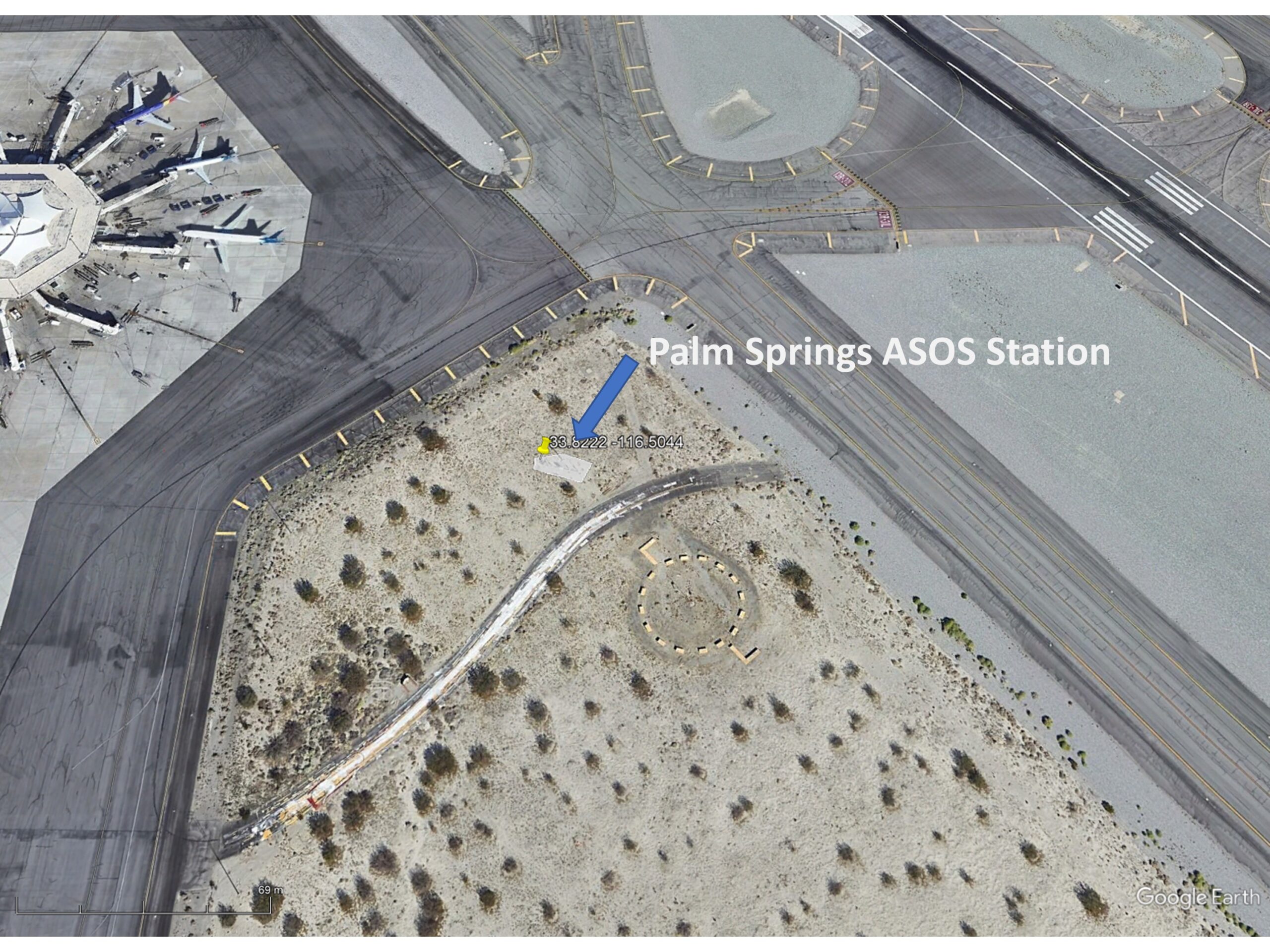
The Palm Springs Airport Weather Observation Site
The following Google Earth image shows the current location of the official ASOS (Automated Surface Observing System) site at the Palm Springs Airport, which recorded an all-time record high temperature of 124 deg. F on July 5 of this year.
What is somewhat amusing is that ASOS meteorological instrument siting guidance favors natural surfaces for placement, but since most of these weather stations are at airports (and since they primarily support aviation weather needs, not climate monitoring needs), the “natural” location is usually right next to runways, aircraft, and paved roads.
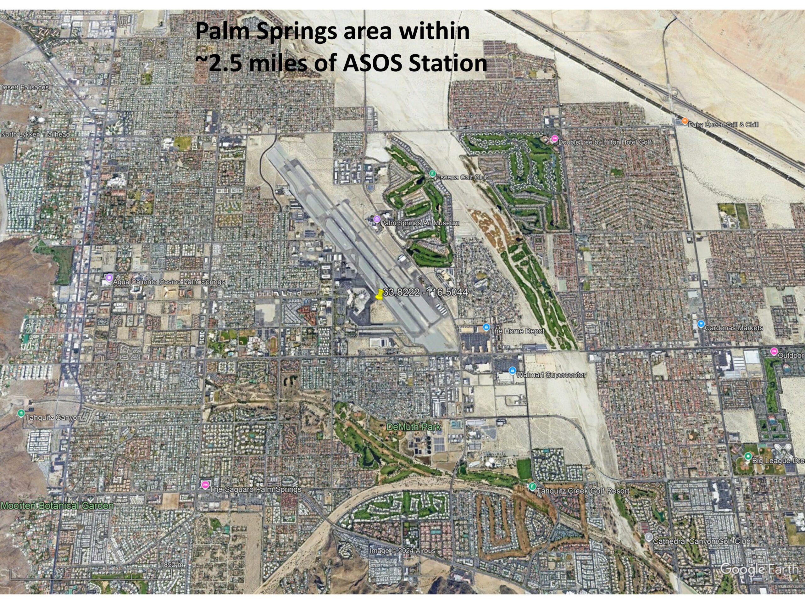
The next Google Earth image is zoomed out to show the greater Palm Springs area, with the ASOS site in the center (click on the image to zoom, then click to zoom more).
Record July Temperatures and Urbanization
It only makes sense that people want to know the temperature where they live, and most of the U.S. population resides in urban or suburban locations. Yet, the temperatures they experience are, probably without exception, higher than before people moved there and started building roads, buildings, and airports.
But what is misleading for those following the global warming narrative is that record high temperatures reported at these locations almost always mention climate change as a cause, yet they have no way of knowing how much urbanization has contributed to those record high temperatures. (Remember, even without global warming, high temperature records will continue to be broken as urbanization increases).
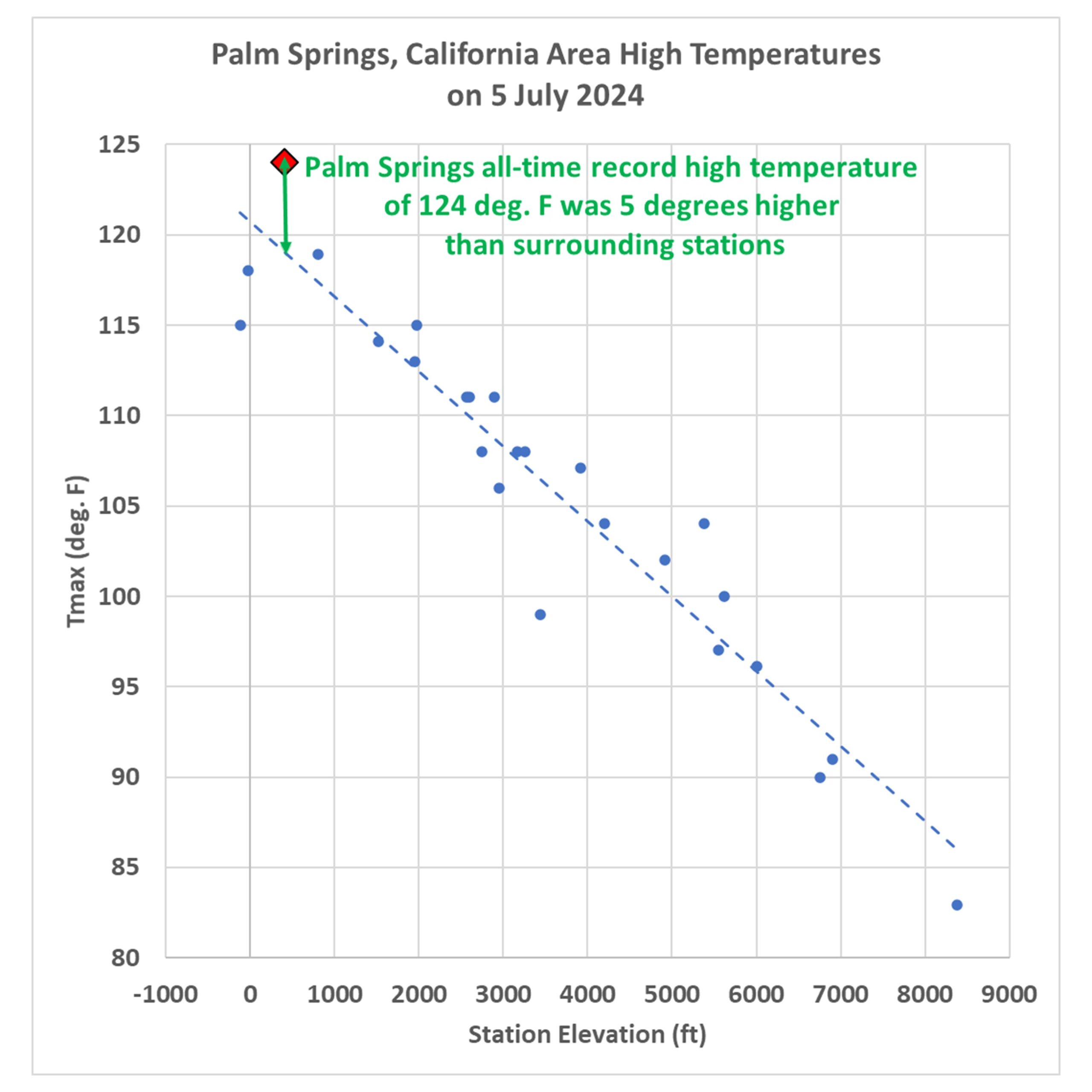
As mentioned above, on July 5, 2024 Palm Springs broke its all-time high temperature record, reaching 124 deg. F. There are 26 other daily GHCN stations within 40 miles of Palm Springs, all with varying levels of urbanization, but even more importantly, at very different elevations. If we plot the high temperatures reported for July 5 at those stations as a function of station elevation, we see that Palm Springs is an “outlier”, 5 degrees warmer than would be expected based upon its elevation-corrected expected temperature (the dashed regression line):
Now, keep in mind that many (if not most) of those 26 surrounding stations have their own levels of urbanization, making them hotter than they would be in the absence of pavement and roofs. So, that 5 deg. F excess is likely an underestimate of how much urban warming contributed to the Palm Springs record high temperature. Palm Springs was incorporated in 1938, and most population growth there has been since World War II.
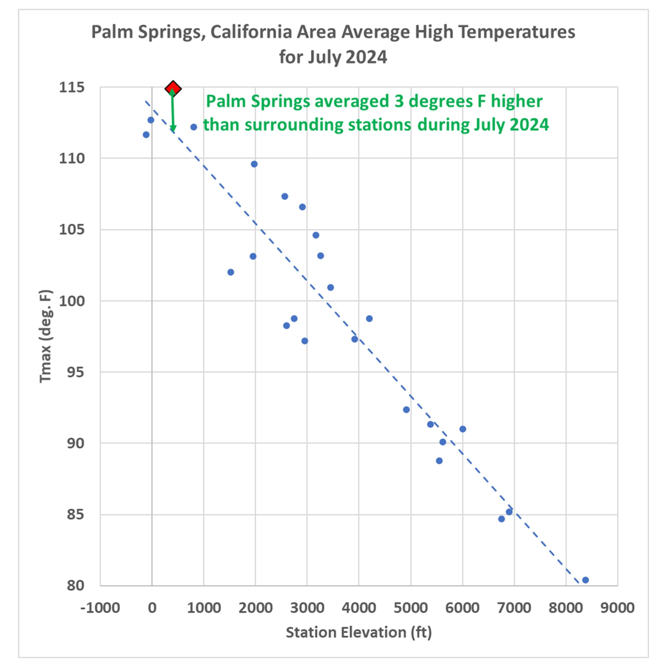
If you are curious how the previous plot looks for the average of all July temperatures, here it is:
For the month of July, Palm Springs averaged 3 deg. F warmer than the surrounding stations (after adjusting for elevation effects, and keeping in mind that most of the *other* stations likely have their own levels of urbanization).
Clearly, Palm Springs has had spurious warming influence from the airport and surrounding urbanization which did not exist 100 years ago. But how much?
Impervious Surface Data as a Surrogate for Urbanization
This blog post is a prelude to a new project we’ve started where we will compare daily (as well and monthly) temperatures to a relatively new USGS dataset of yearly impervious surface coverage from 1985 to 2023, based upon Landsat data. I had previously experimented with a “Built Up” dataset based upon Landsat data, but it turns out that was just buildings. The “impervious surface” dataset is what I believe will have the greatest direct physical connection to what causes most UHI warming: roads, parking lots, roofs, etc. I think this will produce more accurate results (despite being only ~40 years in length) than my population density work (which is, we hope, close to being accepted for publication).

 Home/Blog


