
 Home/Blog
Satellite and Climate Model Evidence Against Substantial Manmade Climate Change (supercedes “Has the Climate Sensitivity Holy Grail Been Found?”)
by Roy W. Spencer, Ph.D.
December 27, 2008 (last modified December 29, 2008)
ABSTRACT
Three IPCC climate models, recent NASA Aqua satellite data, and a simple 3-layer climate model are used together to demonstrate that the IPCC climate models are far too sensitive, resulting in their prediction of too much global warming in response to anthropogenic greenhouse gas emissions. The models’ high sensitivity is probably the result of a confusion between forcing and feedback (cause and effect) when researchers have interpreted cloud and temperature variations in the real climate system. (What follows is a brief summary of research we will be submitting to Journal of Climate in January 2009 for publication. I challenge any climate researcher to come up with an alternative explanation for the evidence presented below…I would love to hear it…my e-mail address is at the bottom of the page.)
1. INTRODUCTION & BACKGROUND
Since computerized climate models are the main source of concern over manmade global warming, it is imperative that they be tested against real measurements of the climate system. The amount of warming these models predict for the future in response to rising concentrations of carbon dioxide in the atmosphere is anywhere from moderate to catastrophic. Why is this?
It is well known that most of that warming is NOT due to the direct warming effect of the CO2 by itself, which is relatively weak. It is instead due to indirect effects (positive feedbacks) that amplify the small amount of direct warming from the CO2. The most important warmth-amplifying feedbacks in climate models are clouds and water vapor.
Cloud feedbacks are generally considered to be the most uncertain of feedbacks, although all twenty climate models tracked by the Intergovernmental Panel on Climate Change (IPCC) now suggest cloud feedbacks are positive (warmth-amplifying) rather than negative (warmth-reducing). The only question in the minds of most modelers is just how strong those positive feedbacks really are in nature. This article deals with how feedbacks are estimated from satellite observations of natural climate variability…and describes a critical error in interpretation which has been made in the process.
Since at this point you are probably dazed and confused about what a ‘feedback’ is, let’s do a simple thought experiment. Imagine you are out in space, observing the Earth, and feeling the radiant energy it gives off from sunlight reflected off of clouds and from the infrared (heat) radiation it emits in proportion to its temperature.
Now imagine that the Earth’s surface and atmosphere suddenly warm by 1 deg. C, everywhere. In this case the Earth would immediately give off an extra 3.3 Watts per square meter of infrared energy (just as a hot stovetop element gives off more infrared energy than a warm one).
This example represents the “no feedback” case…only the temperature has changed in the system, resulting in extra infrared energy being given off, at a rate of 3.3 Watts per square meter for every degree C of temperature increase. But in the real world, any source of warming (or cooling) causes other changes in clouds, water vapor, etc., to occur. These can cause extra warming if they either increase the amount of absorbed sunlight (e.g. fewer low clouds), or reduce the rate of infrared radiation to outer space (e.g. more water vapor, our main greenhouse gas). These warmth-amplifying changes are called positive feedbacks.
Alternatively, cloud and water vapor changes could decrease the amount of absorbed sunlight or increase the amount of emitted infrared energy, thus reducing the warming. This is called negative feedback.
That number (3.3) thus represents the magic boundary between positive and negative feedback. If satellites measure more than 3.3 Watts per square meter given off by the Earth per degree of global warming, that is evidence of negative feedback. If the number is less than 3.3, that is positive feedback. If the number reached zero, that would correspond to a borderline unstable climate system. The 20 climate models tracked by the IPCC have feedbacks ranging from about 0.9 to 1.9 (all corresponding to positive feedback since they are less than 3.3).
The central importance of feedbacks to the global warming issue can not be overstated. How the radiant flows of energy in and out of the Earth system change with temperature is THE most critical piece of knowledge we need in order to predict whether manmade global warming will be benign — or catastrophic. It is obvious that good estimates of feedbacks are needed from our observations of natural climate variability. This would provide the most important test of climate models: do the models exhibit feedbacks consistent with those we observe in nature?
Unfortunately, such testing of the models has been surprisingly difficult. I am now convinced that the main difficulty in diagnosing feedbacks from observations of natural climate variability has been related to the issue of causation when observing cloud behavior. The best way to introduce what I mean by this is with the following question:
When low cloud cover is observed to decrease with warming, is the cloud change the result of the warming, or is the warming the result of the cloud change?
Some will claim that the direction of causation does not really matter, and that all we really need to know is the average relationship between temperature and clouds — but I will show that this is incorrect.
Decreasing low cloud cover caused by warming would be a positive feedback, since it would let more sunlight in. But what if, say, a change in atmospheric circulation patterns caused the decrease in low cloud cover? In that case, warming would be the ‘effect’, rather than the ’cause’. And as we shall see, this can give the illusion of positive feedback — even when negative feedback really exists.
For instance, if the Earth warms by 1 deg C and our satellites measure only 1 watt per square meter of extra radiant energy being given off, since that is less than the magic 3.3 value we might be tempted to say that strong positive feedback is the cause. But this assumes the change in radiant energy is the RESULT of the warming. As we will see, the same result can be obtained if the true feedback number is, say, 6 (strong negative feedback), but most of the cloud change was actually the CAUSE of the warming.
The issue I am raising is not a new one, as there have been general concerns previously published about the diagnosis of feedbacks (e.g. Stephens, 2005; Aires and Rossow,2003). I am merely getting very specific about what has previously been a more general concern.
In the theoretical analysis by Forster and Gregory (2006) of the factors impacting feedback estimation, it was claimed that internal natural variability in clouds would not contaminate the estimation of feedbacks�or that it would, at most, only make feedback estimates from satellite measurements “noisy”, with a variety of diagnosed feedbacks clustering around the “true” feedback value. But as we showed in Spencer and Braswell (2008), something as simple as daily random variations in cloud cover will cause diagnosed feedbacks to not only be ‘noisy’, but also to be biased in the direction of positive feedback.
Here I will show further evidence, from both climate models and satellite data, that this issue is so serious that it might well have caused climate modelers to mistakenly conclude that cloud feedbacks in the climate system are positive when in fact the evidence, when more critically examined, suggests they are negative.
There has also been a persistent concern in the climate research community that feedbacks diagnosed from relatively short satellite datasets, even if they were accurate, might not have anything to do with feedbacks involved in long-term global warming.
Here I will briefly address both of these issues. Specifically, I will show that:
1) the IPCC climate models indicate that short-term and long-term feedbacks in those models are substantially the same, and
2) a simple climate model tuned to mimic recent NASA Aqua satellite observations of global radiative imbalance, sea surface temperatures (SSTs), and tropospheric temperature (Tair) variations, suggests that short term feedbacks in the real climate system are strongly negative.
Taking (1) and (2) together, one must then consider the possibility that current climate models are too sensitive — possibly by a wide margin — and they are therefore forecasting too much global warming and associated climate change in response to anthropogenic greenhouse gas emissions.
2. FEEDBACKS IN THE IPCC CLIMATE MODELS
Feedbacks are not explicitly input into climate models. They are instead the net result of all the different physical processes contained in the models�especially those related to clouds and water vapor. Feedbacks are diagnosed from model output in much the same way as they are diagnosed from satellite measurements of the Earth: by comparing (1) global average temperature variations to (2) global average variations in the radiative balance of the Earth (variations in the approximate balance between absorbed sunlight and emitted infrared radiation averaged over the whole Earth).
The following figure shows yearly- and globally-averaged near-surface (2 meter) air temperature (T2m) variations versus top-of-atmosphere longwave (LW) infrared radiative variations from three IPCC climate models. The yearly averages are plotted every month from the first 60 years of ‘transient’ greenhouse gas experiments in which the radiative forcing from extra carbon dioxide is slowly increased over time.
Plotting yearly averages every month in Fig. 1 allows the time-evolution of the model runs to be visualized, which turns out to be a critical step in the physical interpretation of the models’ behavior.
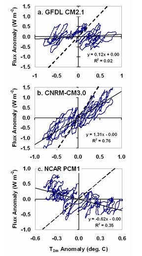
Fig. 1. Sixty years of global average variations in near-surface air temperature versus top-of-atmosphere infrared radiative flux in three of the climate models tracked by the IPCC. See text for details.
We are particularly interested in the linear striations which appear in Fig. 1. I have previously documented these striations in satellite measurements, and argued that their slope corresponds to the strength of feedback in the climate system. Unfortunately, two research papers containing evidence of this were both rejected for publication based upon poor reviews from a single reviewer – a rather unusual basis for total rejection by any science journal.
Well, once again the linear striations appear – but this time in the climate models themselves! And their slopes do indeed correspond to the long term feedbacks (dashed lines in Fig. 1) diagnosed by Forster and Taylor (2006) from these models’ response to anthropogenic greenhouse gas forcing.
In addition to the linear striations, we also see evidence of spiral patterns in Fig. 1. These spirals were seen, to a lesser or greater extent, in all 18 IPCC models we analyzed. More examples of these spiral patterns are seen in Fig. 2 for the CNRM-CM3.0 model.
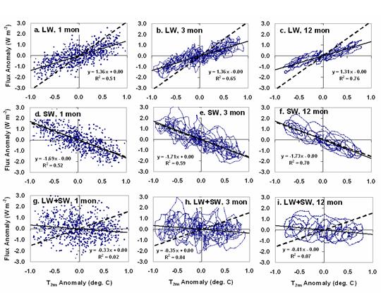
Fig. 2. As in Fig. 1, but for the emitted infrared longwave (LW), reflected solar shortwave (SW) and total (LW+SW) radiative fluxes in the CNRM-CM3.0 model, for various data averaging time intervals.
Note how the raw monthly averages (the panels on the left side of Fig. 2) produce just a ‘cloud’ of points on the graph. Independent yearly averages also produce a cloud of points. It is only when we plot overlapping averages — e.g., yearly averages computed every month — that we see these linear and spiral patterns appear.
Next I will show that the linear striations and spiral patterns can only be explained by feedback and radiative forcing, respectively. In the current ‘forcing-feedback’ paradigm of climate variability, those are the only two kinds of radiative variations possible – forcing and feedback (or, loosely speaking, ’cause and effect’) — and they have distinctly different signatures in the data. There are no other physical explanations for such patterns.
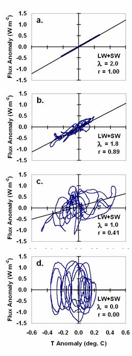 As shown by Spencer & Braswell (2008) radiative feedback can only be accurately diagnosed from satellite data when it is in response to non-radiative forcing of temperature change: primarily variations in evaporation and precipitation. As shown in Fig. 3 (on the right), a simple model whose temperature is forced with only non-radiative forcing (panel a), produces a perfect feedback signal, with the temperature and radiative flux changes falling neatly along a line, the slope of which is the feedback I specified in the model run (2 Watts per sq. meter per degree).
But as increasing amounts of randomly varying radiative forcing is mixed in with the non-radiative forcing (panels b and c), spiral patterns begin to appear, decorrelating the data and reducing the slope of a line fit to the data. Finally, if the forcing is 100% radiative (panel d), then no ‘feedback stripes’ are evident — even though the same feedback (2 Watts per sq. meter per degree) is occurring in all four panels. In this case, the slope of a line fit to the data is zero. And since a total feedback parameter of zero corresponds to a borderline unstable (highly sensitive) climate system, this represents a potentially serious problem when it comes to diagnosing feedbacks from satellite data.
The importance of this can not be overstated. To the extent that natural cloud fluctuations are occurring — as evidenced by spiral patterns in the data — the diagnosis of feedbacks by fitting a line to the satellite data will result in a feedback value biased toward zero. This can be mistakenly interpreted as positive feedback — even if strong negative feedback is operating. I suppose you can call this a ‘false positive’, as sometimes occurs in the medical diagnosis of disease.
3. FEEDBACKS IN SATELLITE MEASUREMENTS OF NATURAL CLIMATE VARIABILITY
Now let’s examine what kinds of temperature-radiative flux relationships are seen in the NASA Aqua satellite data. Plots of the total (reflected solar plus emitted infrared) radiative imbalance versus temperature variability are shown in Fig. 4 at various averaging intervals from five years of satellite measurements of global average SST variations (left panels) and tropospheric temperature variations (right panels). The radiative fluxes come from the CERES instrument, the SSTs from the AMSR-E instrument, and the tropospheric temperatures come from the AMSU-A instrument flying on the NOAA-15 satellite.
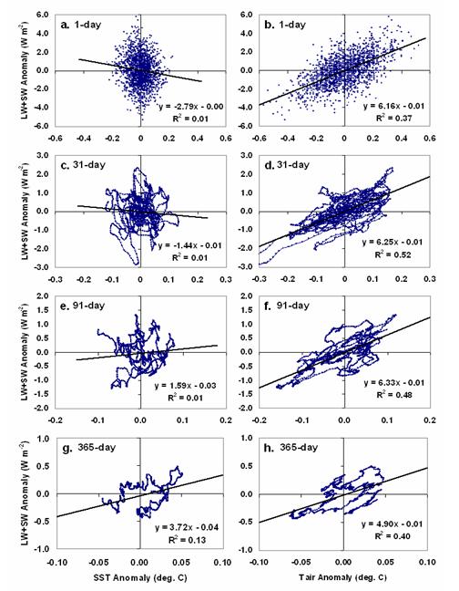
Fig. 4. Aqua satellite-measured total [LW+SW] radiative flux versus SST (left panels) and versus tropospheric temperature (right panels) at averaging times of: (a, b) 1 day; ( c, d) 31 days; (e, f) 91 days; and (g, h) 365 days. (Note that the averaging times now vary vertically, while in Fig. 2 they varied horizontally).
The slopes of the striations seen in the right panels of Fig. 4 (relative to atmospheric temperature) correspond to strongly negative feedback: around 6 Watts per square meter per degree K of temperature change (6 W m-2 K-1). In fact, even though we expect feedbacks diagnosed from the data to be biased toward zero, here the lines fitted to all the data have slopes actually approaching that value: 6 W m-2 K-1. Translated into a global warming estimate, a feedback of 6 W m-2 K-1 would correspond to a rather trivial 0.6 deg. C of warming in response to a doubling of atmospheric CO2.
A couple of the SST plots on the upper left in Fig. 4, however, have very different slopes�but as averaging times get longer, the line slopes also end up corresponding to negative feedback (3.7 W m-2 K-1 in Fig. 4g translates to about 1 deg. C of warming for a doubling of atmospheric CO2).
This very different response for SSTs versus tropospheric temperatures at short time scales is due to the episodic, non-radiative transfers of heat between the surface and atmosphere mentioned earlier (see Spencer et al., 2007, for more evidence of these oscillations).
To demonstrate this physical interpretation, I modified the simple climate model of Spencer and Braswell (2008) to include an atmosphere, an ocean mixed layer, and a deeper ocean layer which slowly exchanges heat with the mixed layer. (These modifications were added one by one, as necessary, to explain characteristics of the satellite data which could not be expalined without those modifications.) The model was driven by radiative and non-radiative forcings that varied randomly in time, having a time scale of days to weeks. The radiative forcing only directly affects the ocean mixed layer, as might be expected with variations in low cloud cover causing varying amounts of absorbed sunlight by the ocean.
In contrast, the non-radiative forcing affects both the mixed layer and the atmosphere, since enhanced evaporative cooling of the ocean surface must be matched by enhanced latent heating of the atmosphere by precipitation systems. As a result, on short time scales, the ocean surface temperature and atmospheric temperaures will be negatively correlated.
The adjustable parameters in the model were then tuned to mimic the lag correlation and autocorrelation structures computed from the five years of daily satellite satellite measurements of tropospheric temperature, sea surface temperature, and radiative flux (see Fig. 5, below, if you are interested in this level of detail).
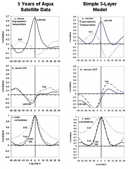
Fig. 5. Lag-correlation and autocorrelations in the five year time series of daily satellite measurments in global oceanic SST, tropospheric temperature, and total (solar +IR) radiative flux.
After this tuning to mimic the satellite measurements, I obtained model behavior (Fig. 6) that looks quite like the satellite data shown in Fig. 4. (If you have a fairly large computer display, you can bring this same web page up in another browser, and compare Figs. 4 and 6 side-by-side.)
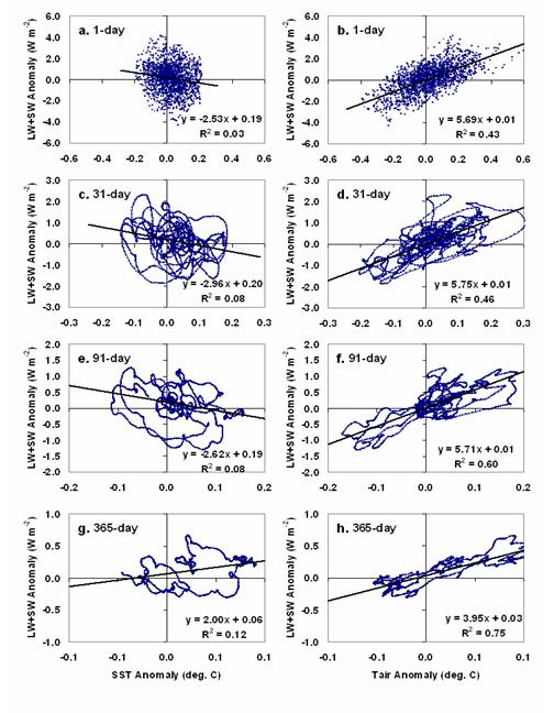
Fig. 6. Five years of variability output from a simple 3-layer climate model tuned to mimic several statistical characteristics of the satellite observations (see text for details)
The important lesson to take from this model simulation is that a strongly negative feedback (6 W m-2 K-1) had to be specified in the model in order to mimic the satellite data in Fig. 4. Note that even though the specified feedback was 6 W m-2 K-1, NONE of the lines in Fig. 6 have a slope that large.
What this means is that the line slopes diagnosed from the satellite data in Fig. 4 might actually be an UNDERESTIMATE of the true feedback occurring, which could be 7 W m-2 K-1 or more.
4. AND FINALLY, FROM NASA’S TERRA SATELLITE…
The data presented above from NASA’s Aqua satellite covered the time period from August of 2002 through August of 2007. But NASA’s Terra satellite also carried a CERES instrument for monitoring radiative fluxes, and those data extend back to March of 2000. This is of particular interest since global temperatures were just beginning a two year long warming trend at that time.
In Fig. 7 (below) I have plotted Terra CERES total radiative flux variations versus NOAA-15 AMSU channel 5 tropospheric temperatures. The data points are 91-day averages plotted every day — just like the Aqua data plotted in Fig. 4g, but now extending back 2.5 years earlier. What is noteworthy in this figure are the clearly displayed feedback stripes, which have an average slope of about 8 W m-2 K-1.
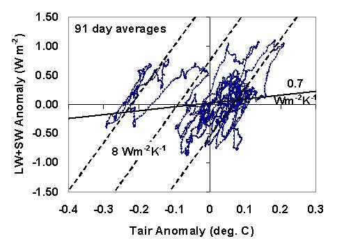
Fig. 7. Terra CERES total radiative flux versus NOAA-15 AMSU tropospheric temperature variations over the global oceans from March 2000 through August 2007.
Together, the CERES data from two separate satellites thus display evidence of what I have used a simple model to explain theoretically: strong negative feedback is observed to occur on shorter time scales in response to non-radiative forcing events (evaporation/precipitation), which are superimposed upon a more slowly varying background of radiative imbalance, probably due to natural fluctuations in cloud cover changing the rate of solar heating of the ocean mixed layer.
5. CONCLUSIONS & DISCUSSION
What I have presented here is, as far as I know, the most detailed attempt to reconcile satellite observations of the climate system with the behavior of climate models in the context of feedbacks. Instead of the currently popular practice of building immensely complex and expensive climate models and then making only simple comparisons to satellite data, I have done just the opposite: Examine the satellite data in great detail, and then build the simplest model that can explain the observed behavior of the climate system.
The resulting picture that emerges is of an IN-sensitive climate system, dominated by negative feedback. And it appears that the reason why most climate models are instead VERY sensitive is due to the illusion of a sensitive climate system that can arise when one is not careful about the physical interpretation of how clouds operate in terms of cause and effect (forcing and feedback).
Indeed, climate researchers seldom (if ever) dig into the archives of satellite data and ask the question, “What are the satellite data telling us about the real climate system?” Instead, most climate research money now is funneled into building expensive climate models which are then expected to provide a basis for formulating public policy. Given the immense effort that has been invested, one would think that those models would be more rigorously tested.
There is nothing inherently wrong with a model-centric approach to climate research…as long as the modeler continues to use the observations to guide the model development over time. Unfortunately, as Richard Lindzen at MIT has pointed out, the fact that modelers use the term “model validation” rather than “model testing” belies their inherent preference of theory over observations. The allure of models is strong: they are clean, with well-defined equations and mathematical precision. Observations of the real climate system are dirty, incomplete, and prone to measurement error.
The comparisons modelers make between their models and satellite data are typically rather crude and cursory. They are not sufficiently detailed to really say anything of substance about feedbacks — in either the models or the satellite data – and yet it is the feedbacks that will determine how serious the manmade global warming problem will be.
And as I have tried to demonstrate here, the main reason for the current inadequacy of such methods of comparison between models and observations is the contaminating effect of clouds causing temperatures to change (forcing) when trying to estimate how temperatures cause clouds to change (feedback). This not a new issue, as it has been addressed by Forster and Gregory (2006, applied to satellite measurements) and Forster and Taylor (2006, applied to climate model output). I have merely demonstrated that the same contamination occurs from internal fluctuations in clouds in the climate system.
The bottom line from the model and observational evidence presented here is that:
Net feedbacks in the real climate system — on both short and long time scales — are probably negative. A misinterpretation of cloud behavior has led climate modelers to build models in which cloud feedbacks are instead positive, which has led the models to predict too much global warming in response to anthropogenic greenhouse gas emissions.
What climate researcher Bob Cess said in a 1997 interview with Science magazine’s Richard Kerr seems to be still true today:
“�the [models] may be agreeing now simply because they’re all tending to do the same thing wrong. It’s not clear to me that we have clouds right by any stretch of the imagination.”
I challenge climate modelers to “validate” their models to the level of detail I have in my comparisons here between satellite observations (Fig. 4 & 5) and a simple climate model (Fig. 5 & 6). Once their climate models can behave in the same way as the satellite observations suggest the real climate system behaves on a year to year basis, then we can revisit how much global warming those models predict for the future. Until that happens, I consider the IPCC climate model forecasts of strong global warming in the coming decades to be completely unreliable for basing policy decisions on.
REFERENCES
Aires, F., and W. B. Rossow, 2003: Inferring instantaneous, multivariate and nonlinear sensitivities for analysis of feedbacks in a dynamical system: Lorenz model case study. Quart. J. Roy. Meteor. Soc., 129, 239-275.
Intergovernmental Panel on Climate Change (2007), Climate Change 2007: The Physical Science Basis, report, 996 pp., Cambridge University Press, New York City.
Spencer, R.W., W. D. Braswell, J. R. Christy, and J. Hnilo (2007), Cloud and radiation budget changes associated with tropical intraseasonal oscillations, Geophys. Res. Lett., 34, L15707, doi:10.1029/2007GL029698.


