ENSO and PDO Explain Tropical Average SSTs during 1950-2013

September 26th, 2013 by Roy W. Spencer, Ph. D.

As most of you are aware, the dominant mode of tropical climate variability is the El Nino Southern Oscillation (ENSO), comprised of El Nino (warm ENSO phase) and La Nina (cool ENSO phase) activity.

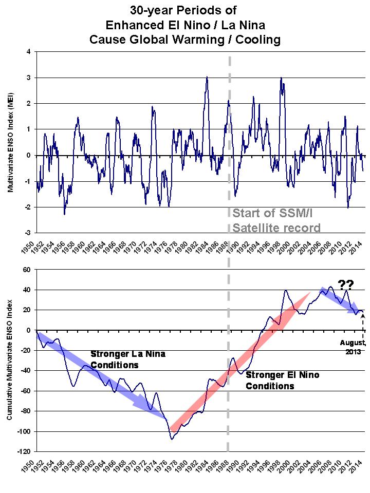
The IPCC has traditionally maintained that El Nino and La Nina activity effectively cancel each other out over time and so ENSO can’t cause multi-decadal time scale warming or cooling. Some of us think this is nonsense, since we know that there are ~30 year periods when El Ninos are stronger, then ~30 year periods when La Nina is stronger.

So, what does 30 year natural climate change have to do with long-term anthropogenic global warming? Well, AGW is can only explain warming over the last 60 years or so, because there weren’t appreciable greenhouse gas emissions before then. And it just so happens that the last 60 years was comprised of 30 years of stronger La Ninas (cool conditions) followed by 30 years of stronger El Ninos (warm conditions). So, it is only “natural” that some recent papers have (finally!) begun to explore the potential role of natural climate fluctuations in explaining at least some of recent warming (or lack thereof).

While our forthcoming paper will address this in a more physically consistent manner, here I will continue this theme by showing just how easy it is to statistically explain tropical sea surface temperature (SST) variations since 1950 with natural modes of climate variability. This is not an entirely new or novel idea, and if someone else has done something very close to the following, consider this independent verification of their calculations. 😉

You can use statistical linear regression (I did it within Excel, the spreadsheet is here) to explain 5-month running average tropical HadSST3 variations as a linear combination of the Multivariate ENSO Index (MEI), the cumulative MEI index since 1950, and the cumulative Pacific Decadal Oscillation (PDO) index since 1950. The original HadSST3 data, and the model fit are shown in the first panel of the following figure, and the model residuals are shown in the second panel (click for larger version; fitted curves are 3rd order polynomials):
HadSST3-tropics-vs-reg-model

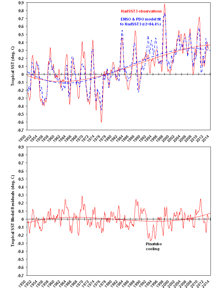
Note the largest excursion in the model residuals (variations the model can’t explain, 2nd panel) is the cooling caused by the Mt. Pinatubo eruption. The linear trends in the observed and model-fitted SSTs are essentially identical.

Of course, the most important (and controversial) aspect of this exercise is explaining the warming trend in terms of the time-accumulation of the MEI index, which would be more than just a statistical artifact *if* persistent La Nina’s early in the record are associated with a net loss of deep-layer ocean thermal energy, and persistent El Nino’s later in the record are associated with a net gain of heat by the ocean. Our paper published next month will show the evidence that this, indeed, happens. The third term in the model equation (time accumulated PDO index) has a smaller influence than the accumulated MEI term, by about a factor of 2.3.

Of course, being a statistical exercise, the above results are far from proof that nature explains everything. From a theoretical perspective, I would expect that increasing CO2 should have some non-zero warming influence.

But as I have mentioned before, the rate of rise in ocean heat content since the 1950s corresponds to only a 1 in 1,000 imbalance in the radiative energy budget of the Earth (~0.25 W/m2 out of ~240 W/m2).

The IPCC’s belief that nature keeps the climate system energy-stabilized to better than 1 part in 1,000 is a matter of faith, not of physical “first principles”.


31 Responses to “ENSO and PDO Explain Tropical Average SSTs during 1950-2013”

Toggle Trackbacks

    • vukcevic says:

      The above may be correct, as long as one accepts that the AMO, the PDO and the ENSO are purely natural oscillations. Such assumption could be made only if the causes are identified with a sufficient degree of confidence. Here I show that the data for the above indices correlate with the data for tectonic activity in the North Atlantic, the North and the (sub)Equatorial Pacific.
      http://www.vukcevic.talktalk.net/APS.htm
      Common driver enhances probability of a casual relationship.

  1. Time you all recognised how it could work:

    http://www.newclimatemodel.com/new-climate-model/

    Simply put:

    Solar variability alters global cloudiness to skew ENSO (and then the other ocean oscillations including AMO) between dominant El Nino (warming) and dominant La Nina (cooling) throughout the millennial solar cycles as seen from Minoan Warm Period to Roman Warm Period to Mediaeval Warm Period to Current Warm Period.

    That solar influence is superimposed on the 60 year PDO which is an internal oceanic cycling periodicity.

    Those solar variations, modulated by a lagging oceanic response shift the climate zones and jets by up to 1000 miles latitudinally in certain regions.

    I doubt that our emissions would shift the pattern by as much as a mile.

    Rebut or concede.

  2. “persistent La Nina’s early in the record are associated with a net loss of deep-layer ocean thermal energy, and persistent El Nino’s later in the record are associated with a net gain of heat by the ocean. Our paper published next month will show the evidence that this, indeed, happens”

    El Nino is a heat discharge process for the oceans so to see a heat gain during a period of dominant El Ninos you have to have more energy entering the oceans than is lost by those El Ninos.

    La Nina is a heat recharge process for the oceans so to see a heat loss during a period of dominant La Ninas you have to have less energy entering the oceans than is gained by those La Ninas.

    The only way to achieve such scenarios is to vary the proportion of solar energy that gets into the oceans.

    That involves cloudiness and albedo changes.

    There needs to be less clouds when the ocean is accumulating energy despite more El Ninos.

    There needs to be more clouds when the ocean is failing to accumulate energy despite more La Ninas.

    We see reduced cloudiness when the sun is more active plus increasing ocean heat content despite more El Ninos (late 20th century).

    We see increased global cloudiness when the sun is less active plus decreasing ocean heat content despite more La Ninas (the current situation is turning in that direction).

    • Kristian says:

      “The only way to achieve such scenarios is to vary the proportion of solar energy that gets into the oceans. That involves cloudiness and albedo changes.”

      No. You can also vary the wind stress across the ocean basin in question, strongly affecting the rate of oceanic energy loss by evaporation. This is in fact potentially a factor of even larger magnitude and influence on the net energy budget than cloud changes. A major switch in the mean level of trade wind strength across the east and central tropical Pacific occurred in 1976/77, when the SOI dropped ‘over night’ and basically stayed at the markedly lower level for the next three decades:

      http://i1172.photobucket.com/albums/r565/Keyell/SOI_zps4a244c80.png

      http://i1172.photobucket.com/albums/r565/Keyell/SOIvslatentampwind_zps8dcdab36.png

      The sudden drop in the pressure differential between Darwin and Tahiti in 1976/77 flattened the east/west thermocline in the tropical Pacific, relatively warming the East and cooling the West. And this extraordinary and basinwide regime shift, best known as the ‘Great Pacific Climate Shift’, kickstarted the modern global warming era.

      • “You can also vary the wind stress across the ocean basin in question, strongly affecting the rate of oceanic energy loss by evaporation”

        I agree, but that is going to involve the changes in jet stream tracks, climate zone positions and cloudiness so it is already factored into my hypothesis.

        • Kristian says:

          Sure. All I’m saying is that you cannot just consider how much energy is coming in. You also need to factor in how much energy is going out per unit of time.

          • Kristian says:

            And a major change in the ‘going out’ part of the equation apparently took place in 1976/77, with the Great Pacific Climate Shift.

          • Agreed.

            However it goes in or comes out it translates into circulation changes.

            The only remaining issue is as to how large is the effect of our emissions on the circulation.

            I guess less than a mile compared to up to 1000 miles for natural solar and oceanic influences.

  3. ren says:

    It can be seen that the oceans absorb heat strongly.
    http://www.ospo.noaa.gov/data/atmosphere/radbud/gs19_prd.gif

  4. ren says:

    Comparison of the temperature in the stratosphere over the equator and solar activity in this cycle.
    http://www.cpc.ncep.noaa.gov/products/stratosphere/temperature/70mb2525.gif
    http://www.solen.info/solar/images/cycle24.png
    It can be seen that the decrease in solar activity causes a drop in temperature.

  5. ren says:

    It is interesting that the low activity decreases the temperature in the stratosphere over the equator and there are changes in temperature over the pole. Above the equator is the strongest Earth’s magnetic field and the weakest ionization by cosmic rays.

  6. Christopher Game says:

    Get me those toys!

  7. Nabil Swedan says:

    Dr. Spencer: Your temperature trend, and others’, show clearly that El-Ninios and La Ninias cancel each other. So is the effect of volcanic events and the 11 year solar cycle. The net heat of natural variability, based on observation, is zero. I cannot immagine how you can prove to the public otherwise.

    • ren says:

      I am convinced that solar cycles through the stratosphere closely with ocean cycles and likely to earthquakes. Studies have shown that these cycles of the Sun can be many.

      Title:
      A Phenomenological Study of the Cosmic Ray Variations over the Past 9400 Years, and Their Implications Regarding Solar Activity and the Solar Dynamo
      Authors:
      McCracken, K. G.; Beer, J.; Steinhilber, F.; Abreu, J.
      Affiliation:
      AA(Institute for Physical Sciences and Technology, University of Maryland), AB(Eawag), AC(Eawag), AD(Eawag)
      Publication:
      Solar Physics, Volume 286, Issue 2, pp.609-627 (SoPh Homepage)
      Publication Date:
      09/2013
      Origin:
      SPRINGER
      Abstract Copyright:
      (c) 2013: Springer Science+Business Media Dordrecht
      DOI:
      10.1007/s11207-013-0265-0
      Bibliographic Code:
      2013SoPh..286..609M
      Abstract

      Two 9400-year long 10Be data records from the Arctic and Antarctic and a 14C record of equal length were used to investigate the periodicities in the cosmic radiation incident on Earth throughout the past 9400 years. Fifteen significant periodicities between 40 and 2320 years are observed in the 10Be and 14C records, there being close agreement between the periodicities in each record. We found that the periodic variations in the galactic cosmic radiation are the primary cause for periods 250 years. The spectral line for the Gleissberg (87-year) periodicity is narrow, indicating a stability of ≈ 0.5 %. The 9400-year record contains 26 Grand Minima (GM) similar to the Maunder Minimum, most of which occurred as sequences of 2 – 7 GM with intervals of 800 – 1200 years in between, in which there were no GM. The intervals between the GM sequences are characterised by high values of the modulation function. Periodicities < 150 years are observed in both the GM intervals and the intervals in between. The longer-period variations such as the de Vries (208-year) cycle have high amplitudes during the GM sequences and are undetectable in between. There are three harmonically related pairs of periodicities (65 and 130 years), (75 and 150 years), and (104 and 208 years). The long periodicities at 350, 510, and 708 years closely approximate 4, 6, and 8 times the Gleissberg period (87 years). The well-established properties of cosmic-ray modulation theory and the known dependence of the heliospheric magnetic field on the solar magnetic fields lead us to speculate that the periodicities evident in the paleo-cosmic-ray record are also present in the solar magnetic fields and in the solar dynamo. The stable, narrow natures of the Gleissberg and other periodicities suggest that there is a strong "frequency control" in the solar dynamo, in strong contrast to the variable nature (8 – 15 years) of the Schwabe (11-year) solar cycle.

    • They don’t cancel on multidecadal timescales such as from one positive phase of the PDO to the next.

      There appears to have been upward ‘stepping’ during the recovery from the LIA and I suspect there would have been downward ‘stepping’ from MWP to LIA.

  8. Dr. Strangelove says:

    In statistical process control, the observed variability must exceed certain threshold in order to trigger a search for unusual/unnatural causes of the deviation. Otherwise, the default is null hypothesis. There is nothing to explain because the deviation is consistent with chance, the expected variability.

    In case of global warming, is the observed temperature trend in past 100 years highly unusual such that we are compelled to reject the null hypothesis? In the national conference on climate change of the National Academy of Sciences, I asked a respected Professor and climate scientist after his presentation – how do you know if the warming is natural or anthropogenic? Can you isolate the anthropogenic effects such as urban heat island effect from the data? He said theoretically it’s possible to detect man-made effects but in reality no we don’t know exactly how much.

    IMO given the uncertainty with temperature data, we cannot reject the null hypothesis. We can propose AGW theories but we may be just looking at statistical artifacts.

  9. Bil Danielson says:

    Dr Spencer, any thoughts regarding the recent NAS study? Not a big fan ofFoxNews, but I did find this article a compelling counter punch.. Which concluded by stating: “Those radical forms of social engineering, it turns out, are the real short-term threat of climate change. And the science-policy community that is pushing them is substituting heated rhetoric for real data that doesn’t support their agenda.”

    http://www.foxnews.com/opinion/2013/09/26/dont-be-fooled-latest-attempt-to-discredit-climate-skeptics-flops/

  10. Thanks, Dr. Spencer.
    I think ENSO and its associated PDO tell almost the whole story. A little greenhouse effect might explain additional warming after the multisecular recovery from the ‘Little Ice Age’ is accounted for.
    Waiting for your new paper.

  11. Fantastic website. Plenty of useful info here. I am sending it to some friends are also sharing in delicious. And naturally, thanks to your effort!

Leave a Reply