Mystery Climate Index #2 Explanation

May 8th, 2015 by Roy W. Spencer, Ph. D.

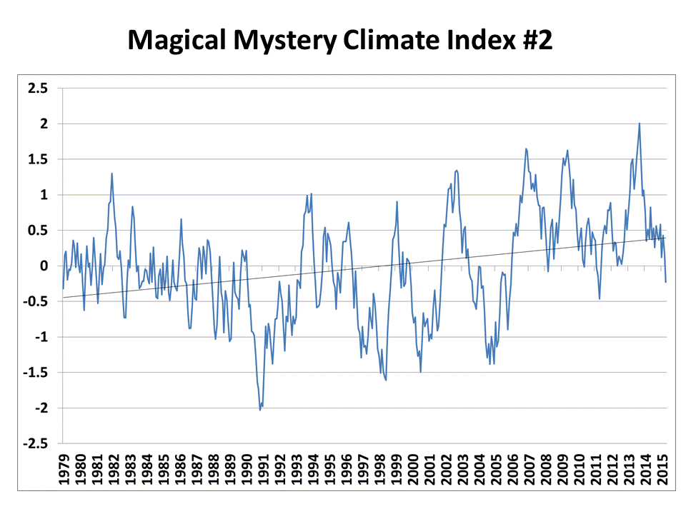
Yesterday I presented this time series of climate data and asked if anyone could determine any physical causes based upon it’s character:

mystery-climate-index-2

I like the example because it shows realistic variability compared to, say, global average temperature variations.

I created it with a very simple function that actually has some basis in how the real climate system operates. Lance Wallace came closest to the right explanation. Bob Tisdale even gave a prediction of how politicians and environmentalists would have used it to call for energy policy changes. 🙂

But the time series, with its multi-decadal warming trend, was created entirely from a monthly series of random numbers. It’s what I call a “constrained random walk”.

How Does this Relate to the Real Climate System?
If you had random monthly cloud variations over the earth, it would cause a monthly random climate forcing as more or less sunlight was absorbed by the system. That effect is cumulative, since the heat is stored by the land and the ocean. So, every month’s value is just the previous month’s value plus a new random number (I used +/-0.5 as the range of random numbers in Excel). BUT…this would just produce a random walk, which almost always wanders away from the average state over time. This is in contrast to the real climate system, which has net negative radiative feedback (the more it warms, the more infrared energy it loses to space, restoring the system to an average state).

You can mimic this negative feedback by just subtracting off 10% of the previous month’s value from the next month’s value. In other words, instead of each month being the previous month’s value plus a random number (which would produce a random walk), use 0.9 times the previous month’s value instead. This is actually an approximation to the time-dependent energy budget equation in a 1D global energy balance model.

The reason for this example is to show that relatively rapid (monthly) forcing in the form of just random cloud variations can cause low-frequency climate variability…even multi-decadal temperature trends. You don’t need variations in solar activity. The reason why is the climate system’s “memory” — its ability to store energy. Certain preferred time scales of temperature variability tend to show up because of certain characteristics of the system — the depth of the ocean mixed layer, the time it takes the tropical atmosphere to overturn, etc.

This kind of variability is contained, to a lesser or greater extent, in all of the IPCC climate models. The cloud variations aren’t really “random” because they have physical causes, but they can seem random because the causes are myriad and complex. This is also the type of simple climate model forcing we used in our papers demonstrating how cloud feedbacks in the climate system have likely been misinterpreted, because researchers tend to assume cloud variations are caused by temperature variations while ignoring causation in the opposite direction.

Thanks to everyone for offering their ideas. I hope you are beginning to appreciate how some of the structure we see in global temperature variations might simply be just nature flipping a coin.


48 Responses to “Mystery Climate Index #2 Explanation”

Toggle Trackbacks

  1. Ed Caryl says:

    It even has El Nios and La Nias!

    That simple illustration falsifies CAGW.

    • Bill says:

      What happens if you plot just the Artic?

      The southern hemisphere hasn’t changed much, but the northern has, due to differences in feedback.

      But we won’t see a chart of the Arctic here, will we?

  2. jimc says:

    Good demonstration that negative feedback is alive and well (and that the strong positive feedback of the IPCC models is bunk).

    • jimc says:

      As Kevin points out, its not as simple as I just said. Different disciplines seem to have different definitions of feedback. Plus multiple feedbacks are woven into the climate system and climate is widely distributed with huge time delays.

      • jimc says:

        How do you model such a thing? The feedback model appeals to an engineer, the constrained random walk seems to give a nice appearance, and I suppose chaos theory could give some appealing curves. In the end, I suspect the climate will always surprise us by just do its thing. But there has to be some cause-and-effect logic worth finding too. Just dont bet the farm on it.

  3. KevinK says:

    Dr. Spencer, nice demonstration of how a simple interaction of random events with some delay of “energy” flowing through a system creates what at times looks like upwards trends, then downward trends and oscillations.

    In electrical engineering what the climate science community refers to as a “feedback” is simply a “reaction” to a change in the state of the system. The term feedback is “reserved” for cases with an amplifier and intentional manipulation of the output by feeding some of the output back to the input of the amplifier. None of the classic electrical feedback analysis methods (Bode, etc.) are appropriately applied to the climate.

    Nice explanation.

    Cheers, KevinK.

    • Paul Aubrin says:

      You say: “The term feedback is reserved for cases with an amplifier and intentional manipulation of the output by feeding some of the output back to the input of the amplifier. None of the classic electrical feedback analysis methods (Bode, etc.) are appropriately applied to the climate.”
      If you consider a system in which the input variable is CO2 concentrations, an open loop transfer function and temperature as output, I see no reason why the general mathematical theory of system should not apply. In which case, the notion of feedback, and all the theoretical tools (diagrams) are valid.

      Any practical stable system has built-in negative feedback.

  4. Ken Gray says:

    Thank you, Dr. Spencer. This is very clear. I took psychology in college but also a year of calculus so I was able to understand it. You do a great service to us voters who never took a class in meteorology or climatology. Please keep up the good communications. You are making a difference. Thanks.

  5. Nicely done. If a random walk can simulate what looks to be a realistic climate metric, complete with El Nino events and La Nina events, it suggests that natural variation and Lorenzian chaos is a much bigger “forcing” than the posited worrisome man-made influences.

    • Curious George says:

      That’s how most IPCC models operate. Throw out any inconvenient run, and you are left with a nice CMIP5 ensemble.

  6. JustAnotherPoster says:

    Our famous stat person did this many many years ago now 🙂

    http://wmbriggs.com/post/257/

    Links to a old but VERY readable paper on it !

    • Thanks, Just.
      The Gordon paper, and the Briggs post are both very interesting. Both do great damage to the AGW hypothesis.

    • Aaron S says:

      Cool article. Points out another interesting learning for me. It is NOT random noise if a data set has been selected based on desired traits. Given unlimited potential runs or selecting a subset of a longer run by definition you will match whatever pattern you desire. So is there a difference in drawling the pattern you want and waiting for a suitable one to emerge?

      • ferdberple says:

        indeed it is not random noise, due to auto-correlation. it is power series noise (1/f noise).

        i did this same study some years back using excel to generate the series. the interesting thing for me is that if you leave off the numbers on the axis, you cannot tell if you are looking at the past 30 years or 30 thousand years of 30 million years.

  7. JustAnotherPoster says:

    The “External” shocks quote here….

    http://journals.ametsoc.org/doi/abs/10.1175/1520-0442%281991%29004%3C0589%3AGWAAMO%3E2.0.CO%3B2

    could be El Ninios, Volcanoes etc.

  8. Aaron S says:

    This is a great learning, we humans always look for patterns… easy to think we see them in noise. After all that is the brains job… to turn noisy observations to a mental model. I am confused by the report of fft yielding spectral peaks in this noise and will have to look at it more. Thanks for the experiment and humbling reminder.

    • jimc says:

      Hi Aaron. I dont know how to transmit a copy of it to you. I did a 256 pt transform of the first 256 smpl (you have to stick to powers of 2). I got (relative) peaks in bins 4, 8, 12, and 15 which would be periods of 5.33, 2.57, 1.77, and 1.38 yrs. I can only imagine the frequencies are harmonics of RWSs sample generation frequency. If you dont have fft already installed in your Excel, its in the analysis toolpak which you can install and use via the MS office helps.

  9. Aaron S says:

    Can you explain or better quantify what was a constrained random walk?

    • as I explained in words, the temperature anomaly at time i is simply 0.9 times the temperature anomaly at time [i-1], plus a new random number.

      T(i) = 0.9*T(i-1) + R(i)

      If 0.9 is replaced by 1.0, it’s just a random walk. Using a value less than 1.0 tends to force the long-term average toward a constant value, rather than “walking away”. So, I call it a “constrained random walk”.

      This is the same as the Planck Effect that stabilizes the global temperature, and is contained in all climate models: Increasing temperature is naturally reduced by increasing IR energy loss to outer space.

      Without that stabilizing effect, the climate system would be unstable to perturbations.

      Any positive feedbacks in the climate system have to be less than the negative “feedback” Planck Effect for the system to remain stable. (IPCC types don’t call the Planck Effect a feedback, leading to endless confusion among engineers.)

      • Paul Aubrin says:

        “IPCC types dont call the Planck Effect a feedback, leading to endless confusion among engineers”

        Indeed, the choice of the IPCC to borrow a word, used in a well established mathematical theory, and to use it with a substantially different meaning, is a source of unnecessary confusion in the scientific (or technical) community. Some climate scientists are also known for the use of their personal statistical methods rather than well established ones.

        Yet using the same vocabulary as other scientists offers a lot of advantages, as the present example, based on random walks and its arcsin law, proves.

  10. Lance Wallace says:

    Thanks. I guess my prize is to see my name in lights.

    Here is a graph of the first differences. Looks very random indeed.

    https://dl.dropboxusercontent.com/u/75831381/Magical%20Mystery%20First%20Differences.jpg

    A great textbook on probability theory is Feller, which I studied in 1957 at Caltech. He showed that as time goes on, the random walk spends longer and longer times in negative or positive space. So people looking at a single realization of a random walk will interpret it as a force pushing it in one direction.

    • ferdberple says:

      indeed. we tend to thinks the result will hover around zero, but it will not.

      there is money to be made in this, because the gullible will tend to think that once negative the results should go positive to try and “balance out” the result.

      but in reality, once the result goes negative, the odds are increased that it will remain negative, simply because the starting point for the rest of the numbers is now negative.

      whatever came before no longer has meaning, thus the fact that it is negative cannot make it go positive.

  11. Lance Wallace says:

    Here is the graph of Feller’s illustration of the ever-longer waves associated with a random walk

    https://dl.dropboxusercontent.com/u/75831381/Feller%20random%20walk%20graph.pdf

    By the way, I just now looked up the book and it seems to have cleared copyright protection–you can download the 1950 3rd edition in its entirety here.

    http://alg.csie.ncnu.edu.tw/~ykshieh/b1.pdf

    I used the random appearance of the first differences to guess that Roy’s graph was a random walk. However, I missed the coefficient of 0.9 that would serve to limit the “straying” from the initial condition. I wonder if there is a way to estimate the coefficient, or in general terms, to distinguish a random walk from a “constrained random walk”

  12. Mike Bromley the Kurd says:

    This is at least elegant..I think Neil deGrasse Tyson uses an upside-down dartboard.

  13. Thanks, Dr, Spencer.
    Good learning experience.
    Yes, a random walk constrained by a chaotic system comprising many feedback control regulators.
    Albedo changing clouds and storms, and snow-cover on land, sea ice forming and breaking up, are a few possibilities.

  14. lemiere jacques says:

    but first a random walk implies divergence, so at best the climate is “chaotic between boundaries..

    andnever forget that such a thing that the average temperature of “lower troposphere” must look a little chaotic, because the very unphysical nature of such a thing, it is not even a close system…and because the circulation of air is messy ( molecules of airs follows what mus be seen as a random walk!)… this must be reflected in global temperature .

    second on a finite period a random walk may result in any mathematical curve..just a matter of luck..

    a lot of macroscopic things look random , all are by very nature of microscopic though the aim game is to try to find out the miraculous laws that appears in macroscopic systems..

    • Paul Aubrin says:

      “second on a finite period a random walk may result in any mathematical curve..just a matter of luck..”

      No. Not in “any” possible mathematical curve.

      “a lot of macroscopic things look random , all are by very nature of microscopic though the aim game is to try to find out the miraculous laws that appears in macroscopic systems..”

      When are such macroscopic laws to be discovered? Will they even be discovered? And, worse, how will such laws of atmospheric physics be validated, using either the very short instrumental record, or the much more uncertain indirect proxy data?

  15. Gordon Robertson says:

    “…which has net negative radiative feedback (the more it warms, the more infrared energy it loses to space, restoring the system to an average state)”.

    Not only that, negative feedback is the natural state of real processes due to losses. If there were no losses, real processes could produce a positive feedback leading to perpetual motion.

    In a reply to Roy above, Paul Aubrin states, “IPCC types dont call the Planck Effect a feedback, leading to endless confusion among engineers.

    It’s the same with the usage of ‘positive feedback’ by climate alarmists of the modeling persuasion. Engineers don’t understand their usage of positive feedback because PF requires amplification independent of the feedback.

    Some people are under the impression that PF causes amplification. It does not. In systems incorporating PF, the PF signal is a fraction of the output signal fed back in phase with an input signal. When the combined signal is amplified, the output signal increases exponentially unless steps are taken to control the growth.

    The equation for PF in physics contains a gain component.

    One example is G = A/(1-AB)

    Where G is the overall system gain, A is the amplifier gain, and B is the feedback signal.

    Since B is taken as a fraction of A, then AB < 1. If AB = 1, the system is unstable.

    The equation above leads to a gain that is always increasing, provided AB < 1.

    If AB << 1, then 1 – AB is a large fraction like 0.9, and the gain will increase more slowly.

    Also, the equation G = A/(1-AB) is not the true representation of PF as used in an electronic amplifier. In the term AB, as defined, A is a fixed value as in the specified gain of a transistor, which is relatively constant. For example, a typical transistor gain may be specified as 100, meaning it amplifies the input base current by 100.

    However, a transistor is not a magical device that can provide gain out of nothing, it requires an external power source to supply both it's base current and output collector current. therefore, a transistor is really a transducer that enables a low input current to enable a higher output current in the collector circuit, supplied by a power supply.

    This is important because A is that fixed gain in the transistor. In a real positive feedback system, AB becomes the amplified signal not the fixed gain. Therefore A is increasing during each cycle of the output signal.

    There are no process in the atmosphere that produce such a gain or satisfy an equation for PF like the one above. That is especially true when it comes to amplifying heat, which is the average kinetic energy of atoms in a substance.

    How can you increase kinetic energy without increasing solar energy?

    • jimc says:

      Hi Gordon, I think what he implies above and said outright in Blunder is that to a climatologist, positive and negative feedback are different than what you and I are used to. I.E., if you increase the CO2 by a certain amount and everything else stays the same, the lower temperatures must rise to force the same radiation out the TOA. But, the higher lower level temperatures will actually cause other changes more clouds possibly. These other changes (once everything is stabilized again) can add to (positive feedback) the increased temperature or subtract from (negative feedback) the original increase of temperature. I think the IPCC says the CO2-alone-increase will get multiplied by some ridiculous factor (I seem to remember something like 5). RWS thinks it may be closer to 0 and doesnt rule out a slight negative.

      • jimc says:

        I should have said that the CO2-alone-increase is a theoretical (calculated) value. I’m not giving a good explanation here.

      • Doug Cotton says:

        There is absolutely no valid physics that can be applied to show any reason as to why greenhouse gases like water vapor and carbon dioxide supposedly cause Earth’s surface temperature to be warmer. They do the opposite.

        There is still AU$5,000 (about US$4,000) on offer to the first in the world to prove the physics and the evidence that I have presented to be substantially incorrect.

        See http://climate-change-theory.com

  16. Doug Cotton says:

    Roy – the natural climate cycles are discussed at http://climate-change-theory.com and there are compelling reasons as to why these must be being regulated by planetary orbits.

    Carbon dioxide has nothing to do with any warming of Earth’s surface. Increasing water vapor very clearly causes lower surface temperatures.

  17. Layman Lurker says:

    Interesting post Roy. I am convinced that understanding the “memory” of the climate system is the key to understanding the system itself. Fitting autocorrelation functions to temperature series might yield some insights into this. For example, the ACF of tropical oceans looks much different then ocean ACF’s at higher latitudes. It stands to reason due to the energy imbalance between tropics and poles – tropics are continuously losing heat to the poles (therefore shorter memory).

  18. vfiore says:

    Interestingly, a one-dimensional random walk never escapes its starting point. more precisely, the root mean squared displacement remain finite in 1d; 2d is wishy-washy (log divergence, so almost no divergence 😉 and in 3d the walk can (in principle) go to infinity during its evolution. so no runaway if the effective dimensionality of the problem is 1 or 2.

    • Joel Shore says:

      I think you are either confusing this with another process or another measurement other than root mean squared displacement. For a random walk, the root mean squared displacement goes like sqrt(t) independent of the dimension.

      There are some differences in dimensions for such issues as the probability of the walk returning to the origin after some time, but in all dimensions the mean squared displacement is proportional to the square root of the number of steps.

  19. Dr. Strangelove says:

    Roy

    Try this related exercise. Reproduce the observed global temperature trend from 1950-2014 using a random walk function. This is easy. You can reproduce the trends of different data sets (GISS, Hadcrut, NCDC, BEST) You can do this using Excel’s random number generator. I bet you can get the trends in less than 100 simulation runs. You can calculate the probability of getting the trend by chance

    P = 1/N

    P is the probability; N is the number of runs until the desired trend is obtained

    Example, you got the trend after 20 runs. P = 1/20 = 0.05
    In physical science, the gold standard for statistical significance is 5 sigma or 1/3,500,000. If you get the trend only after 3.5 million runs, you can rule out the event (real world temperature trend) occurred by chance.

  20. wayne says:

    Doc, I am finding the parameters you stated don’t necessarily need to be so large (or small).

    I assume you used something like T(month) = Tbase + var(month-1)*autocorr_rate + (rand()*2-1)*var_rate. Is that pretty much the same you are using? The rates are both bound between 0 and 1. When autocorr_rate is one, that is just a normal random walk and as you said can wander anywhere.

    You say 0.9 and 0.5 but I am finding with a plot in excel of 12000 months that just 0.999 and just 0.05 for example stays in the range of about 2C about Tbase (I set it at 288.15K) no matter how many times you press F9 to get a new random plot. It is interesting how those two parameters affect the temperature range and the noise levels.

    So what would that 0.999 signify physically?

    Very nice article!

    • Dr. Strangelove says:

      It means a monthly variation of 0.001 C can give 2 C change in temperature over 1,000 years. Try 0.1 C over 100 years. What is the change in temperature? Do a regression over 100 years to get the trend line. What is the probability P = 1/N

      • Dr. Strangelove says:

        What answer are you talking about? I did not give any answer, just the parameters for you to try. Why are you surprised with your result? 3.5 C change in 50 years is not impossible. I think that’s a maximum deviation, not the 50-year trend.

        Your 1 million Kelvin is impossible at 0.1 K variation per month, the maximum deviation is 1200 K over 1,000 years and that’s statistically improbable and physically impossible.

    • wayne says:

      Strangelove, you are way off base on that answer but I appreciate your guess. Even in just 600 months the temperature sometimes goes all of the way from 286.5K to 290K so that is not merely some rate per month. Upon further toying with this releation that parameter seems definitely related to the noise range. The other affects how loose the constraint is but they affect each other. I’ll give you the way to duplicate my spread sheet below, only takes setting seven cells and then dragging two down to 12000 if you want to see a simulation of climate over 1000 years. Take the time to see yourself, Takes but a few minutes to have it up and running. Hit F9 on excel to force a new random graph.

      Params:
      Cell A1 = 288.15
      Cell A2 = 0.05
      Cell A3 = 0.999

      Initial:
      Cell C1 = 0
      Cell D1 = C1+$A$1

      Rest of cells:
      Cell C2 … on down = C1*$A$3+(RAND()*2-1)*$A$2
      Cell D2 … on down = C2+$A$1

      Highlight C2 & D2 and drag them down to 12000. Plot column D. Especially toy with A2 and A3 dictating the constraints on this constrained random walk that Dr. Spencer laid out… very interesting!

    • wayne says:

      Also that parameter definitely has to do with controling the system’s stability. A setting of exactly one is a classic random walk but when ever above one, like at 1.001 or 1.0001, you get runaway results like wandering to 1 millon Kelvin or -20000 K, totally instable.

  21. Ansgar John says:

    Great relevant for investing on the stock exchange as well. Malkiel says stock prices move in a random walk. Warren Buffett (Ben Graham) say in the short term the market is a voting machine, in the long term a weighing machine.
    The right term is a constrained random walk. Does that make sense ? http://sinaas.blogspot.nl/2013/02/value-investing-margin-of-safety-beta.html

    • Dr. Strangelove says:

      The stock market isn’t random but it is too complex to be predictable in the short term (daily or weekly). It can be simulated by a random walk function because it appears to be random much like tossing a coin is completely deterministic but we all believe it’s random. Our guess is approximately true.

  22. Ulric Lyons says:

    “The reason for this example is to show that relatively rapid (monthly) forcing in the form of just random cloud variations can cause low-frequency climate variabilityeven multi-decadal temperature trends. You dont need variations in solar activity.”
    +
    “The cloud variations arent really random because they have physical causes..”

    You do need solar variations in solar activity, there is no internal solution to natural variability, and there never will be. The elephant in the room is wind driven ocean modes rather than cloud variability, particularly the global AMO signal.

  23. Jim Medlin says:

    You could take a linear combination of periodic events (different periods and amplitudes) and get a similar function. This would be a Fourier synthesis type of addition. What are there… 10 or 20 different cyclic events that produce the temperatures observed in nature? For example, we see daily and yearly temperature variations. Then there are the 11-year sunspots and the 30-year Pacific Ocean thing, etc. In geology, temperature variations with periods of thousands to millions of years are interpreted from relative sea level changes.
    It would be interesting to calculate the Fourier transform (EXCEL routine) from your time series and see what frequencies and phases are present in your “random” model.

  24. Ray says:

    How does Excel generate it’s “random” numbers?
    Does it generate truly random numbers or “pseudo” random numbers by some mathematical formula?

Leave a Reply to Dr. Strangelove