Updated: Low Climate Sensitivity Estimated from the 11-Year Cycle in Total Solar Irradiance

June 4th, 2010 by Roy W. Spencer, Ph. D.

NOTE: This has been revised since finding an error in my analysis, so it replaces what was first published about an hour ago.

As part of an e-mail discussion on climate sensitivity I been having with a skeptic of my skepticism, he pointed me to a paper by Tung & Camp entitled Solar-Cycle Warming at the Earth’s Surface and an Observational Determination of Climate Sensitivity.

The authors try to determine just how much warming has occurred as a result of changing solar irradiance over the period 1959-2004. It appears that they use both the 11 year cycle, and a small increase in TSI over the period, as signals in their analysis. The paper purports to come up with a fairly high climate sensitivity that supports the IPCC’s estimated range, which then supports forecasts of substantial global warming from increasing greenhouse gas concentrations.

The authors start out in their first illustration with a straight comparison between yearly averages of TSI and global surface temperatures during 1959 through 2004. But rather than do a straightforward analysis of the average solar cycle to the average temperature cycle, the authors then go through a series of statistical acrobatics, focusing on those regions of the Earth which showed the greatest relationship between TSI variations and temperature.

I’m not sure, but I think this qualifies as cherry picking — only using those data that support your preconceived notion. They finally end up with a fairly high climate sensitivity, equivalent to about 3 deg. C of warming from a doubling of atmospheric CO2.

Tung and Camp claim their estimate is observationally based, free of any model assumptions. But this is wrong: they DO make assumptions based upon theory. For instance, it appears that they assume the temperature change is an equilibrium response to the forcing. Just because they used a calculator rather than a computer program to get their numbers does not mean their analysis is free of modeling assumptions.

But what bothers me the most is that there was a much simpler, and more defensible way to do the analysis than they presented.

A Simpler, More Physically-Based Analysis

The most obvious way I see to do such an analysis is to do a composite 11-year cycle in TSI (there were 4.5 solar cycles in their period of analysis, 1959 through 2004) and then compare it to a similarly composited 11-year cycle in surface temperatures. I took the TSI variations in their paper, and then used the HadCRUT3 global surface temperature anomalies. I detrended both time series first since it is the 11 year cycle which should be a robust solar signature…any long term temperature trends in the data could potentially be due to many things, and so it should not be included in such an analysis.

The following plot shows in the top panel my composited 11-year cycle in global average solar flux, after applying their correction for the surface area of the Earth (divide by 4), and correct for UV absorption by the stratosphere (multiply by 0.85). The bottom panel shows the corresponding 11-year cycle in global average surface temperatures. I have done a 3-year smoothing of the temperature data to help smooth out El Nino and La Nina related variations, which usually occur in adjacent years. I also took out the post-Pinatubo cooling years of 1992 and 1993, and interpolated back in values from the bounding years, 1991 and 1994.
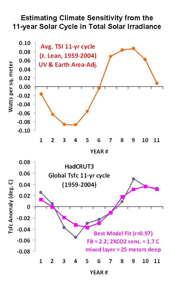
Note there is a time lag of about 1 year between the solar forcing and the temperature response, as would be expected since it takes time for the upper ocean to warm.

It turns out this is a perfect opportunity to use the simple forcing-feedback model I have described before to see which value for the climate sensitivity provides the best fit to the observed temperature response to the 11-year cycle in solar forcing. The model can be expressed as:

Cp[dT/dt] = TSI – lambda*T,

Where Cp is the heat capacity of the climate system (dominated by the upper ocean), dT/dt is the change in temperature of the system with time, TSI represents the 11 year cycle in energy imbalance forcing of the system, and lambda*T is the net feedback upon temperature. It is the feedback parameter, lambda, that determines the climate sensitivity, so our goal is to find a value for a best value for lambda.

I ran the above model for a variety of ocean depths over which the heating/cooling is assumed to occur, and a variety of feedback parameters. The best fits between the observed and model-predicted temperature cycle (an example of which is shown in the lower panel of the above figure) occur for assumed ocean mixing depths around 25 meters, and a feedback parameter (lambda) of around 2.2 Watts per sq. meter per deg. C. Note the correlation of 0.97; the standard deviation of the difference between the modeled and observed temperature cycle is 0.012 deg. C

My best fit feedback (2.2 Watts per sq. meter per degree) produces a higher climate sensitivity (about 1.7 deg. C for a doubling of CO2) than what we have been finding from the satellite-derived feedback, which runs around 6 Watts per sq. meter per degree (corresponding to about 0.55 deg. C of warming).

Can High Climate Sensitivity Explain the Data, Too?

If I instead run the model with the lambda value Tung and Camp get (1.25), the modeled temperature exhibits too much time lag between the solar forcing and temperature response….about double that produced with a feedback of 2.2.

Discussion

The results of this experiment are pretty sensitive to errors in the observed temperatures, since we are talking about the response to a very small forcing — less than 0.2 Watts per sq. meter from solar max to solar min. This is an extremely small forcing to expect a robust global-average temperature response from.

If someone else has published an analysis similar to what I have just presented, please let me know…I find it hard to believe someone has not done this before. I would be nice if someone else went through the same exercise and got the same answers. Similarly, let me know if you think I have made an error.

I think the methodology I have presented is the most physically-based and easiest way to estimate climate sensitivity from the 11-year cycle in solar flux averaged over the Earth, and the resulting 11-year cycle in global surface temperatures. It conserves energy, and makes no assumptions about the temperature being in equilibrium with the forcing.

I have ignored the possibility of any Svensmark-type mechanism of cloud modulation by the solar cycle…this will have to remain a source of uncertainty for now.

The bottom line is that my analysis supports a best-estimate 2XCO2 climate sensitivity of 1.7 deg. C, which is little more than half of that obtained by Tung & Camp (3.0 deg. C), and approaches the lower limit of what the IPCC claims is likely (1.5 deg. C).


20 Responses to “Updated: Low Climate Sensitivity Estimated from the 11-Year Cycle in Total Solar Irradiance”

Toggle Trackbacks

  1. John Lohman says:

    Excellent work! (and I suspect we could explain 90% of HadCRUT variation using TSI, its impact on cloud cover, and ocean circulation).

  2. Andrew says:

    There have been different types of analyses done on the solar cycle signal. One approach has been to try and use ENSO and aerosol indeces to estimate the temperatrue changes unrelated to the TSI variations by multiple regression, EG Douglass and Calder:

    Determination of the Climate Sensitivity of the Earth to Solar Irradiance David H. Douglass, B. David Clader Geophysical Research Letters 10.1029/2002GL015345. 2002

    What seems to be the first major problem with the Camp and Tung analysis is that if it were true that the amplitude of the solar cycle signal supported climate model sensitivities, then climate models would presumably show the same amplitude of a cycle. This is not the case, as the variability of the solar cycle is extremely damped by the long response time of sensitive climate models. Somehow, Camp and Tung think that the response time is very short but the sensitivity is very high. That is physically unreasonable.

    The second problem is that they essentially assume that the apparent solar cycle component is caused by the TSI alone. This leaves out the possibility of a coincidence (spurious correlation) or some amplifier of the solar cycle variations. I don’t want to start a debate about the controversial cosmic ray hypothesis, but Camp and Tung do implicitly exclude it from their analysis, and anything which is not known.

    Also, just a gripe: There were no measurements of TSI in the 50’s and 60’s! That part of the TSI data is proxy based and may not be reliable. There is even debate about how to stitch the measured satellite data together, see acrim . com for example.

  3. Carl Chapman says:

    I think I’ve figured out how this AGW nonsense started.

    Someone calculated the feedback factor to be 3 or 4, so an initial change of 1 degree would be magnified to give a final change of 3 or 4 degrees. But they left out a “/”. It should have been 1/3 or 1/4, so doubling CO2 to give an initial change of 1.2 degrees Celsius would give an insignificant final rise of about 0.3 or 0.4 degrees Celsius.

    I’m joking, but if any of the scammers want to use that excuse rather than admitting they were part of a huge grant driven scam, that’s ok.

  4. christopher Game says:

    Dear Roy, \

    I am away from home, just glancing at things in an internet cafe.

    This is is really the right stuff. I am surprised that the errors are not made too great by the smallness of the signal, but I think this is really sound stuff.

    It is, however, a serious methodological error to simply average out the el Nino kind of thing, since you know it exists. To average it out is to greatly weaken the accuracy of the method. The correct thing is to estimate it explicitly and remove the estimated effect perhaps by subtracting the estimate. We may say, in the language of E.T. Jaynes, that the el Nino kinds of things are “nuisance variables”, and should be integrated over to remove their irrelevant interfering effects. Larry Bretthorst is a top expert who would know with great skill how to do this.

    But using the sunspot cycle is a very very good way to go because it is NOT SRICTLY PERIODIC, and this means that every cycle contains information not present in other cycles.

    And this is really using an external driver. It is of course ENTIRELY DIFFERENT from thinking about the balance between absorbed solar radiation and OLR, which are both internal variables. The present method has no direct information about the degree of absorption and should be combined with an analysis of the reflected solar radiation and the OLR, which can both be measured, I think, and are both internal state variables. If their noise level of measurement is low enough, this should provide you with really hard-core dynamical information, the real stuff. There are standard methods for this kind of analysis.

    The point is that the feedback from earth to sunspot cycle is entirely negligible.

    Great Stuff.

    Yours sincerely,

    Christopher

  5. Craig Goodrich says:

    There is a (relatively) new Scafetta paper linked at WUWT which shows a strong correlation between planetary orbits (principally Jupiter and Saturn, the Big Boys) and the 60-year cycle identified with the PDO. Would backing out PDO effects from your model change the sensitivity?

    Off topic: I’m really not sure that the terms “forcing” and “feedback” are useful in a system as complex as climate, as long as we keep the causality arrows pointing in the right direction.

    For example, suppose Svensmark’s cosmic ray > cloud formation hypothesis is true. (I personally like it.) Then when the solar wind reduces low-level high-energy rays, the rays are a feedback, but when we pass through the galactic plane or a spiral arm, where cosmic rays greatly increase in density, the flux is a forcing.

    Moreover, given the complexity of climate processes, it is likely that we will find that Process A affects Process B, but B has consequences that affect A after a certain lag. Which is the feedback?

    So perhaps it would be better to simply talk about interrelated processes, rather than using the forcing-feedback technobabble.

    • Anonymous says:

      Very likely there is NO direct link between the 20 and 60-70 year PDO cycles and the orbital periods of Jupiter and Saturn. What you are seeing is a dierct link between the PDO and the 20.3 and 62 year Lunar/solar tidal cycles. The

      It just happens that the Lunar/solar tidal cycles are indirectly linked with the orbital periods of the Jovian planets (primarily Jupiter and Saturn).

  6. Andrew says:

    Craig Goodrich-“when the solar wind reduces low-level high-energy rays, the rays are a feedback”

    How so? Feedback refers to changes that are caused by the temperature change initially caused by something else that reinforce or dampen it. The solar wind is not caused by the Earth’s temperature changes.

  7. maxwell says:

    Roy,

    thanks for the analysis. It seems physically reasonable, though I have to admit I have not yet checked out the Tang paper.

    Quick note. Do you think you could plot the results of running more physically-intuitive model with a high climate sensitivity? It would be nice to visualize how they differ from the results with a low climate sensitivity.

    Also, as the sensitivity gets higher, does the lag time between the solar and temperature change get smaller?

    Thanks for the explanation.

  8. Andrew says:

    Maxwell-Roy will probably want to answer this himself, but I just want to say regarding the question:

    “Also, as the sensitivity gets higher, does the lag time between the solar and temperature change get smaller?”

    I would say that based on my knowledge of the physics of these models, this is almost the opposite of how it would be expected to work. A more sensitive system normally responds more slowly to perturbation.

  9. […] Spencer on climate sensitivity and solar irradiance Posted on June 5, 2010 by Anthony Watts Updated: Low Climate Sensitivity Estimated from the 11-Year Cycle in Total Solar Irradiance […]

  10. Anonymous says:

    This paper also got a value close to 1.7, or 1.9 +/- 1

    http://www.ecd.bnl.gov/pubs/BNL-80226-2008-JA.pdf

    Given the multitude of papers that put the value higher that 1.5, that statement in the IPCC report seems to be jsutified.

  11. Guy says:

    It seems like coming up with the increase in degrees celsius per doubling of CO2 levels is the type of thing that could be done in a laboratory setting.

  12. maxwell says:

    Andrew,

    ‘A more sensitive system normally responds more slowly to perturbation.’

    I think this depends on how close to particular system’s resonances one is with the perturbation. In the case of the climate, it seems hard to model such resonances.

    So we have to compute the response with the simple model Dr. Spencer is discussing here. I was just wondering if he had done that already.

    Thanks for the reply.

  13. MapleLeaf says:

    Dear Dr. Spencer,

    Thanks for this interesting analysis, and for opening up the comments section.

    I’m intrigued that you did not mention that Tung et al. (2008, GRL) published a paper in which they used four datasets (two reanalysis products (NCEP, ERA-40) and two in-situ (GISS, HadCRUT3)) and TSI data to estimate the transient climate response. They established the existence of a response to the solar cycle in all four SAT datasets (using linear discriminant analysis) above the 95% level of confidence. TSI data from Lean et al. (1995) from 1959 to circa 2005 was used in their analyses.

    Tung et al. (2008) then calculated the transient climate response (TCR, which is what you seem to be estimating here) for the HadCRUT3 data to be +2.5 K, with a corresponding equilibrium climate sensitivity (ECS) of +3.8 K.

    Unless I am missing something, it is critical to note that the number you arrive at (+1.7 K) seems to be for the TCR and not the ECS. Yet the numbers from the IPCC which you cite are for the ECS (not the TCR) and the ECS is estimated to be higher than the TCR by a factor of 1.5 (Tung and Camp 2008, JGR; Stott et al. 2006, J. Climate).

    Would it be possible for you to provide some error bars for your estimate of TCR, or at least quantify the uncertainty? It appears that your TCR value is close to that of Tung et al. (2008), and that there may even be some overlap once uncertainty is considered.

    It did not escape my attention that your value for TCR is more than three times higher than the estimate made by Lindzen (~ +0.5 K). If I may be so bold, perhaps a more appropriate title for your post would be “Transient climate response estimated from the 11 year cycle in TSI is at lower bound of values reported in the IPCC”.

    PS: Have you any plans to publish this?

    Hat tip and thanks to LHarris.

  14. George E. Smith says:

    Well I don’t see any TIME factor in your analysis. If doubling CO2 causes the temperature to increase; does that happen in the few tens of microseconds it takes to get an LWIR photon from the surface to a few km high CO2 molecule; or does the temperature change not happen until 800 years before the CO2 increase that caused it.
    Most real (rather than fictional) physical processes have a propagation delay between cause and effect.

    So what delay do you use in your “Climate sensitivity” analysis; in order to get a true logarithmic temperature resonse to CO2 changes.

    Personally, I prefer the mechanism that is implicit in the results of Frank Wentz et al, in SCIENCE for July-7 2007; “How much More rain Will Global Warming Bring ?”

    They report that a 1deg C rise in mean global surface Temperature results in a 7% increase in total global evaporation; a 7% increase, in total atmospheric water content,; and a 7% increase in the total glohbal precipitation.
    Implicit in that result; but not stated specifically by Wentz is an increase (maybe about 7%) in the total global precipitable cloud cover; presumably in the form of increased area; increased optical density; and increased cloud perisistence time; or some combination of all three.

    But no way can you get 7% morre rain and snow; without having considerably more global cloud cover; and increases in cloud cover over climatic time scales (how about 30 years) ALWAYS cause cooling from increased blocking of incoming solar spectrum radiation to the ground (or water).

    So I favor a “model” where H2O completely regulates the temperature of the earth. Vapor leads to warming (of the atmosphere), but maybe cooling of the ground from loss of solar energy to the atmosphere; and clouds lead to cooling by increased albedo reflection off cloud tops plus increased absorption of additional solar energy; so that IT ALWAYS GETS COLDER IN THE SHADOW ZONE.

    So if I add a bit more CO2 OR A BIT MORE TSI; I simply end up with a small increase in total global cloud cover; which blocks a bigger fraction of the TSI.

    And if Svensmark’s Cosmic Rays, make cloud formation a little easier; then I get more cloud cooling for less surface warming (mostly of the ocean).

    You guys are making it all far too complicated.

    IT’S THE WATER !

  15. Roger says:

    I don’t think there is much point to beating on the solar variability issue post 1970. It is well known and documented that the solar contribution during this period depends critically on the solution to the “ACRIM” gap problem (see for example N. Scafetta, Empirical analysis of the solar contribution to global mean air surface temperature change. Journal of Atmospheric and Solar-Terrestrial Physics(2009),doi:10.1016/j.jastp.2009.07.007), which is the result of the gap in the TSI data due to the Challenger disaster. The bridging of that gap has been the subject of much debate. However, there is also much to suggest that a combination of global temperature changes due to (1) unforced secular ocean cycles as proposed by Roy; (2) forcings by TSI variations; and (3) forcings by GHGs via a small climate sensitivity (less than or of the order of 1 deg C) gives a very good empirical accounting of 20th century change.

  16. Dan Kirk-Davidoff says:

    Dr. Spencer’s fit looks a little funny- for one thing it obviously doesn’t capture that maximum or minimum temperature very well. I thought that was curious so I tried two things. First, I used the sum of the square error as the criterion for best fit, instead of correlation. In that case, the best fit is for a feedback parameter of 1.57 (or a sensitivity of 2.4°C). At that value of lambda, the correlation is 0.95 instead of 0.96 at lambda = 2.2, but the sum of the squared error is 0.0142 instead of 0.0172 (a much better fit).

    Second, I tried using a mixed layer depth of 20 m, instead of 25 m. Now the lambda with the lowest sum of squared errors is lambda = 1.49 (Climate Sensitivity = 2.51), with r = 0.9607. The highest correlation occurs at lambda = 1.63 (r = 0.9618).

    There’s no way to simultaneously optimize the correlation in both lambda and Cp: it’s always a trade-off (higher heat capacity implies lower sensitivity). But it’s easy to find the best fit in terms of sum of the squared errors: there’s a clear minimum at 18 m mixed layer and lambda = 1.47, which implies a climate sensitivity of 2.54. On the same arbitrary scale, the sum of the squared errors is 0.0090, substantially better than the fit that Dr. Spencer obtains. At that location, the correlation coefficient is 0.9617.

    Now, I just grabbed the numbers for Tsi and Tsfc from Dr. Spencer’s plot, and implemented his model in matlab.
    Roy- have I made some error?

  17. Hi Dr Roy,
    A couple of observations on your analysis:

    1) If you average the temperature data over 1/3 of the solar cycle length, you get a curve which matches the TSI data nicely, and shows an amplitude of variation in the region of 0.2C over the solar cycle rather than the 0.08 you found. I believe the tendency of el nino to occur away from the peak of the solar cycle, often soon after minimum, and the tendency for la nina to occur at the peak of the solar cycle flattens the curve of the global temperature response to insolation, and leads to an underestimation of the solar influence on temperature.

    2) You were criticised by Ray Pierre Humbert some time ago for using an ocean heating depth of 1000m for your simple model, and he said 25m was more like it. My calcs on the amount of heat-energy the ocean must have absorbed to account for the steric component of sea level rise 1993-2003 coupled with a calculation of the drop-off in temperature from surface to thermocline show you were right! Heat-energy must be mixed down to much greater depths around 1000m, probably by lunar tidal action over a longer timescale, perhaps due to the changing max declination dragging water latitudinally and causing overturning due to coriolis effect.

    3)Great work, keep it up! Please let us know what result you get with 0.2C variation and 1000m ocean mixing.

  18. Roger says:

    It is doubtful that TSI is an accurate rendition of the actual forcing. It may be a factor of 5-7 too low due to an as yet unidentified amplification mechanism ( For example, N. Shaviv JOURNAL OF GEOPHYSICAL RESEARCH, VOL. 113, A11101, doi:10.1029/2007JA012989, 2008. Roy in fact notes that his analysis does not include the Svensmark cosmic ray mechanism, which may or may not be the culprit. Furthermore, a series of time series analyses by Scafetta and West indicates a significantly larger role of solar variability over the centuries than can be accounted for by TSI alone. Therefore the actual climate sensitivity may be signficiantly lower, and it may be more reasonable to consider the value using TSI alone as an upper limit.

Leave a Reply