Warming in Last 50 Years Predicted by Natural Climate Cycles

June 6th, 2010 by Roy W. Spencer, Ph. D.

One of the main conclusions of the 2007 IPCC report was that the warming over the last 50 years was most likely due to anthropogenic pollution, especially increasing atmospheric CO2 from fossil fuel burning.

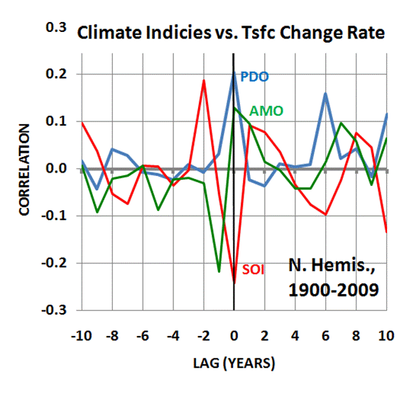
But a minority of climate researchers have maintained that some — or even most — of that warming could have been due to natural causes. For instance, the Pacific Decadal Oscillation (PDO) and Atlantic Multi-decadal Oscillation (AMO) are natural modes of climate variability which have similar time scales to warming and cooling periods during the 20th Century. Also, El Nino — which is known to cause global-average warmth — has been more frequent in the last 30 years or so; the Southern Oscillation Index (SOI) is a measure of El Nino and La Nina activity.

A simple way to examine the possibility that these climate cycles might be involved in the warming over the last 50 years in to do a statistical comparison of the yearly temperature variations versus the PDO, AMO, and SOI yearly values. But of course, correlation does not prove causation.

So, what if we use the statistics BEFORE the last 50 years to come up with a model of temperature variability, and then see if that statistical model can “predict” the strong warming over the most recent 50 year period? That would be much more convincing because, if the relationship between temperature and these 3 climate indicies for the first half of the 20th Century just happened to be accidental, we sure wouldn’t expect it to accidentally predict the strong warming which has occurred in the second half of the 20th Century, would we?

Temperature, or Temperature Change Rate?
This kind of statistical comparison is usually performed with temperature. But there is greater physical justification for using the temperature change rate, instead of temperature. This is because if natural climate cycles are correlated to the time rate of change of temperature, that means they represent heating or cooling influences, such as changes in global cloud cover (albedo).

Such a relationship, shown in the plot below, would provide a causal link of these natural cycles as forcing mechanisms for temperature change, since the peak forcing then precedes the peak temperature.
Predicting Northern Hemispheric Warming Since 1960
Since most of the recent warming has occurred over the Northern Hemisphere, I chose to use the CRUTem3 yearly record of Northern Hemispheric temperature variations for the period 1900 through 2009. From this record I computed the yearly change rates in temperature. I then linearly regressed these 1-year temperature change rates against the yearly average values of the PDO, AMO, and SOI.

I used the period from 1900 through 1960 for “training” to derive this statistical relationship, then applied it to the period 1961 through 2009 to see how well it predicted the yearly temperature change rates for that 50 year period. Then, to get the model-predicted temperatures, I simply added up the temperature change rates over time.

The result of this exercise in shown in the following plot.
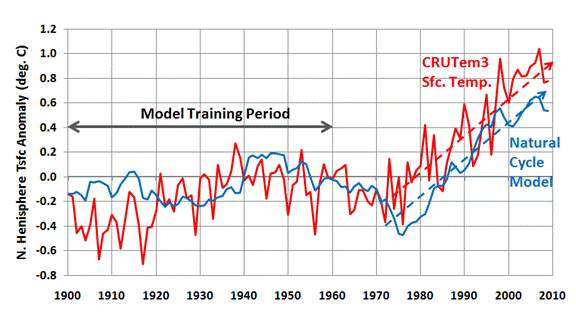
What is rather amazing is that the rate of observed warming of the Northern Hemisphere since the 1970’s matches that which the PDO, AMO, and SOI together predict, based upon those natural cycles’ PREVIOUS relationships to the temperature change rate (prior to 1960).

Again I want to emphasize that my use of the temperature change rate, rather than temperature, as the predicted variable is based upon the expectation that these natural modes of climate variability represent forcing mechanisms — I believe through changes in cloud cover — which then cause a lagged temperature response.

This is powerful evidence that most of the warming that the IPCC has attributed to human activities over the last 50 years could simply be due to natural, internal variability in the climate system. If true, this would also mean that (1) the climate system is much less sensitive to the CO2 content of the atmosphere than the IPCC claims, and (2) future warming from greenhouse gas emissions will be small.


68 Responses to “Warming in Last 50 Years Predicted by Natural Climate Cycles”

Toggle Trackbacks

  1. Andrew says:

    The nature of the Atlantic Multidecadal Oscillation does not seem, to me, to exclude the possibility of being contaminated by a AGW signal in itself. It’s just detrended Atlantic SST. So it’s not clear to me if that’s going to be entirely “natural”. And of course it isn’t independent of the variable it is a predictor of.

  2. Andrew says:

    Oops, sorry, AMO is independent in origin from what it is predicting, I didn’t realize that was land surface temps.

  3. Bret says:

    What do the next 50 years look like according to your model?

  4. Andrew says:

    Bret, the model relies on observaional indices to make statistical “predictions”. It doesn’t have the ability to be extended into the future, as the future PDO, SOI, and AMO haven’t yet been observed for obvious reasons.

  5. Tim says:

    I don’t understand why ENSO and unforced cloud cover changes are discussed as two distinct phenomena. They could be simply two different aspects of the same physical mechanisms.

  6. James Davidson says:

    CO2 levels in 1890 were 290 ppmv. ( Siple ice core.) Current levels ( Mauna Loa ) are 388 ppmv ( round it up to 390 ppmv ) for an increase of 100 ppmv over the last 120 years. The mistake a lot of people seem to make is to treat these as whole numbers, instead of what they are- the numerators of fractions. In 1890 CO2 constituted 290 millionths of the atmosphere, and this has now risen to 390 millionths of the atmosphere – an increase of 100 millionths. To express this as a fraction, multiply by 100, for an answer of 0.01%. If someone in 1890 had decided that CO2 levels should be kept constant and had succeeded 120 years later to within one hundredth of one percent, they would think they had done pretty darn well. I really cannot believe that such a small increase can have had ANY effect on global warming, and as Dr Spencer has shown, natural variation is a more likely candidate.

    • Anonymous says:

      Hi Dr. Spencer,

      I discovered this article following a link to the previous article on Watts Up With That. I found this one much more interesting!

      Such a high degree of correlation between land surface temperature change and major recurring sea surface temperature oscillations seems only reasonably explained by cause/effect linkage.

      I have what may be a naive question that others might have too. What makes you say the SST oscillations are the cause rather than the effect?

      One thing that might make this more compelling is to overlay CO2 concentration onto the graph where, I suspect, the fit won’t be very good. That way, although it doesn’t identify which is cause and which is effect, it would certainly make a case for CO2 not being a cause. The only thing we really need to debunk is CO2 being the bogeyman before we rush headlong into an economically crippling world war against CO2.

      I don’t have a problem with figuring out where the climate is heading in the coming centuries but when we’re talking about scrubbing plant food out of the atmosphere at hideous expense it seems like the cure is far worse than the disease. We need to be damn certain the disease is worse than the cure before we do that. In this case I don’t think we’re even sure there is a disease to say nothing of knowing its cause and cure.

    • William C. Hyland says:

      I have always had serious doubts about measuring CO2 concentrations in ice, as CO2 enjoys a very active chemical life in water ice. I have not read any convincing description of how the researchers have ensured that the CO2 concentrations in the ice cores have been calibrated for dispersal rates, chemical interactions with contaminates, etc. I have also observed that ice cores, while they are stored in conditions that keep them from melting, are not isolated from the present atmosphere of either the storage facility of of the open air when they were collected.

  7. Miroslav Pavlí?ek says:

    I have committed some data analysis as I lived on it. I am not qualified for climate research but used to analyze money. In spite of it I consider the CO2 warming models something out of sound mind. If someone used a SW for $1,000 to apply it for the temperature time series a prefabricated utility would give him decomposition to a trend, seasonal components and a fluctuation residuum. The analyst could be so stupid to omit the regular variations but the SW wouldn’t omit them and each ARIMA algorithm could provide better prediction then the IPCC models. If there are external values that can explain the time series their explanation power could be tested and measured with co-integration tests etc. If there are values like some seasonal indexes or astronomical values that are really associated with the temperature they must be involved into each phenomenological model and they are worthy to be studied while seeking an explanation model though we don’t know how the explanation works yet. If there is an external value with measurable effect less then fluctuation then no one will waste his effort to test causation.

    Why they don’t buy SPSS instead of their models for billions? Why they seek hypothetical omnipotence of CO2 without a co-integration test of its statistical effect?

  8. Bob Tisdale says:

    Dr. Spencer: As you’re aware, the SOI is a sea level pressure index, and it’s inversely related to SST anomalies of the central and eastern equatorial Pacific, but I see no mention of your having inverted the SOI data in your model. You may wish to add a note to that effect.

    Also, why not simply use NINO3.4 SST anomalies, since the SOI (inverted) and NINO3.4 SST anomalies do not correlate perfectly?

    I went through a similar exercise a while back and only needed to create a scaled running total of NINO3.4 SST anomalies to reproduce the basic global temperature anomaly curve:
    http://i39.tinypic.com/2w2213k.jpg
    To me this indicates that the rise in Global Temperature anomalies could reflect the oceans integrating the effects of ENSO. Further illustrated in this post:
    http://bobtisdale.blogspot.com/2009/01/reproducing-global-temperature.html

    And last, regarding the PDO, through what mechanism would the PDO raise and lower global temperatures? The PDO has been shown in numerous papers to lag ENSO, and Newman et al found that it was dependent on ENSO on all timescales:
    http://www.cdc.noaa.gov/people/gilbert.p.compo/Newmanetal2003.pdf

    The PDO and the North Pacific SST anomalies (north of 20N) are not one and the same:
    http://i43.tinypic.com/29fp8ad.jpg

    The PDO bears no similarity to detrended North Pacific SST anomalies:
    http://i42.tinypic.com/17pev8.jpg

    So I’m curious how the PDO could raise and lower global temperatures since it really represents the pattern of SST anomalies in and only in the North Pacific, north of 20N. On the other hand, NINO3.4 SST anomalies have a “multidecadal” component, which can be seen if they’re smoothed with a 121-month filter…
    http://i43.tinypic.com/33agh3c.jpg
    …and the mechanisms through which ENSO raises and lowers global temperatures are known.

    Regards

    • Bob:
      Yes, the SOI regression coefficient was negative, while the PDO and AMO coefficients were positive. This should have been obvious from the first figure in my post.

      The degree to which one of the climate indicies is (or is not) correlated to another, or lagged in time versus another, is interesting, but not necessary for what I am demonstrating. All I am hypothesizing is that these indicies (the PDO, AMO, and SOI) have associated with them non-feedback changes in the radiative budget of the Northern Hemisphere….probably due to circulation-induced changes in albedo due to clouds.

      If this is not the case for one or more of the climate indicies, then the multiple linear regression procedure will assign little or no weight to that index. The possibility of an accidental statistical relationship is greatly reduced by the fact that I trained with pre-1960 data, to then explain the post-1960 warming: an independent test.

      -Roy

      • Anonymous says:

        Dr. Spencer, what effect would including the Indian Ocean Dipole and the more recently identified ENSO Modoki have on your modelling?
        Also would modelling the southern hemisphere be better for correlating natural cycles if the southern hemisphere is perhaps less influenced by human habitation?

        johnd

  9. Christopher Game says:

    This looks like an estimation of the nuisance variables for the total solar irradiation (TSI) effect on climate temperature. The obvious step is now to remove these effects from the time series and again look for the TSI effect. The method of lagged correlations you have used here is perhaps better than using an assumption that the TSI effects is 11-year periodic. Will Alexander has found that a 22-year cycle is nearer to periodicity, and reveals things not seen with the 11-year assumption. But better to let the data speak for themselves, and don’t assume periodicity, but work with the lagged correlation method of the present post. What about a cross-correlogram or two?

  10. johnd says:

    Dr. Spencer, I hope I’m not doubling up, I submitted a question earlier but it hasn’t appeared on the blog. Being new here I’m not sure how the system works.
    My question was regarding the Indian Ocean Dipole (IOD) and the more recently identified ENSO Modoki and how they would correlate if inputted to your modelling.
    I also asked whether modelling the southern hemisphere would show better correlation for these natural climate cycles.

    Thank You.

    • I only included the three most obvious indicies of climate change. The more one includes, the more it will look like an exercise in curve fitting.

      As I understand it, ENSO Modoki is an intermediate state between El Nino and La Nina, so it should be implicit in the SOI index.

  11. johnd says:

    Sorry, I see that the earlier one is now here. Please delete one or the other.
    Thanks

  12. Roger says:

    Very interesting.
    Tsonis et al GEOPHYSICAL RESEARCH LETTERS, VOL. 34, L13705, doi:10.1029/2007GL030288, 2007 have shown that there exist points in time when the decadal ocean cycles synchonize and desynchonize. The cycles they consider are the PDO, the North Atlantic Oscillation NAO (similar to the AMO), the ENSO Index, and the North Pacific Oscillation NPO. These cycles constitute an interconnected complex network of global extent. They model the behavior as a complex system comprised of coupled anharmonic oscillators and identify three points in time during the 20th century (c. 1910, 1940, 1970) when the sychonization underwent a major shift, and these times of course correspond with significant changes in temperature trend. The point is that it may be possible to relate their findings to the parameters you derived from the calibration period, perhaps including air temperature as an additional oscillator. I have found one of the coauthors (Sergey Kravtsov) very responsive and helpful in correspondence with him a couple of years ago.

    Finally I can’t resist but observe that having calibrated the system during the early part of the century you do not get a “divergence problem” afterward.

  13. Dave Springer says:

    If you shift the training window around does it still reproduce the rest of the record accurately?

  14. John McLean says:

    See also the paper that I wrote with Professors Chris de Freitas and Bob Carter, available via http://www.agu.org/pubs/crossref/2009/2008JD011637.shtml.

    We showed that average global temperature anomalies (UAH MSU) correspond well to the SOI (calculated according to the Troup method) of 7 months earlier, except during ad hoc periods of cooling due to volcanic eruptions near the western Pacific, and we show good reasons for the time lag.

    For anyone who claims that the paper was refuted I refer ou to http://scienceandpublicpolicy.org/images/stories/papers/originals/agu_censorship.pdf in which we show that the claims were without foundation. The criticism was focused on the calculation of the 7-month time lag not whether the time lagged SOI corresponded well with the temperature, or at least as well as can be expected when various short-term forces influence temperature and the SOI.

  15. AlanG says:

    Roy, any climate model must ultimately explain past temperatures. It needs to accommodate known changes in forcings and produce the right temperatures. I think a good test would be to run a model for today and for the Holocene optimum when solar forcing was significantly higher. If the model produces the right temperatures then and now then the model feedbacks will look convincing. We know the Sahara was much wetter then. This can only come about if there is more cloud cover giving more rain.

    Your theory about cloud albedo variability looks right to me. It can easily accommodate large changes in solar or other forcings. The Holocene optimum article in Wikipedia says ‘maximum Northern Hemisphere heating 9,000 years ago when axial tilt was 24° and nearest approach to the Sun (perihelion) was during boreal summer. The calculated Milankovitch forcing would have provided 8% more solar radiation (+40W/m²) to the Northern Hemisphere in summer’. If that much forcing only produces a small (NH) temperature rise then the climate must be insensitive.

    • But I would argue that we DON’T know the forcings, not if we ignore internal circulation changes as potential forcings (where by “forcing” I mean top-of-atmosphere radiative imbalances caused by anything other than feedback).

      That’s why I don’t like using the Milankovitch cycles for anything…we don’t know what internal forcings were going on at that time. Just because our most accurate estimates of long-term forcing come from planetary tilt and orbit characteristics doesn’t mean those are the only drivers (or even main) drivers of the climate system. That’s akin to thinking CO2 is the main driver today simply because it’s the one thing we know most accurately.

  16. Tom Skilling is the best! says:

    @AlanG wrote:

    > The Holocene optimum article in Wikipedia says ‘ …

    On a topic as complex and deep as climatology, I’m sorry but Wikipedia is not an authoritative reference. You post is thus noise.

    @johnd wrote:

    > … the more recently identified ENSO Modoki …

    Identified by who? When? How? Why? What? Has there been any peer review about the ENSO Modoki or is this so-called “discovery” a half baked attempt at some scientists somewhere trying to become famous and make a name for themselves? Don’t fall in love with too many phantom teleconnections! (oops, silly me, as a scientist am I not supposed to be skeptical about so-called new discoveries? Form your hypothesis and then try do destroy it into smithereens!).

    @Bob Tisdale:

    On your blogspot.com blog, why do you have your hand out asking for a tip (I.e., “Donations … Tips are now being accepted”)? That is very tacky and by doing so you’re only going to fuel people like John Coleman (visionary of The Weather Channel whose father was a Ph.D) who purports that IPCC Ph.D scientists are banding together in their gospel-like view of AWG because they want money to get their research funded and that’s their motivation for AWG scare tactics (as if they are colluding and forming a conspiracy). It just looks really really bad for a scientist to have his/her hand out asking for donations. Please reconsider modifying your blog HTML.

    @Roy:

    How is it that all or nearly all IPCC scientists have missed temperature change rate considerations in their research? I have my doubts that IPCC suffers from “group think” because its not as if they are all joined at the hip in a tribe that professes the same “corporate” culture. However, I allow for the possibility of tribal-like banding by the IPCC scientists because its human nature to want to belong to a group and it might be very hard to override such human neural wiring.

    • johnd says:

      Tom Skilling, regarding the ENSO Modoki, do some research and bring yourself up to speed.

    • Gator says:

      The IPCC report is not written by scientists. The scientists involved submit their work to govermental reviewers who heavily edit the final report. In the past there have been scientists who have sued the IPCC to have their names removed, because their work was so terribly misrepresented in this “intergovernmental” report. This is not a scientific study.

  17. pochas says:

    Dr. Spencer,

    Your analysis conforms to Scafetta’s 60 year cycle, whereby the 1900 – 1960 pattern, representing a full 60 year cycle, would be expected to repeat.

  18. Andrew says:

    Hey, off topic, but Roy, can you confirm my mathematical intuition on a feedback question?

    Defining Feedback in the following way:

    dT=dT0/1-f

    would then the ratio of radiation flux in response to temperature relate to the value of the feedback factor in the following way:

    dF/K=-3.3(f)+3.3

    Meaning that halving the planck response (the 3.3) would yield a feedback factor of .5 and a sensitivity of twice the no feedback response? And then a response of twice the planck reponse would indicate a sensitivity half that of the zero feedback case.

    Do I have this about right?

  19. Joseph P. Martino PhD says:

    Having degrees in both statistics and physics, I try to look beyond correlations in data (not saying you don’t). The thing that bothers me a bit about your analysis is the use of rates as explanatory variables. In reality, temperatures are physical phenomena. Rates of temperature change are not. They are mathematical constructs. Do you have any idea of how a rate of change of temperature could be an explanatory variable?

    • the heat budget equation for the climate system, or of a pot of water on the stove, is:

      dT/dt = [forcing-feedback]/Cp

      where Cp is the heat capacity of the system. Yes, temperature is a primary state variable, but if you want to examine WHY IT CHANGES, you need to deal with the change rate of temperature.

      Now, if all of the temperature changes represent an equilibrium response, you can do it without a time rate of change term….but the climate system is NEVER in a state of equilibrium.

  20. ldlas says:

    What do you get when you take into account the attribution of the eruptions of volcanoes like Agung, El Chichon and Pinatubo on the temperature?

  21. vukcevic says:

    Northern Hemisphere temperatures trend follows closely the Arctic, with a possible few years phase difference.
    Correlation between variation in the Earth’s magnetic field and the Arctic anomaly is very convincing, but physical relationship as yet unknown.
    http://www.vukcevic.talktalk.net/NFC1.htm

  22. Turboblocke says:

    “The AMO signal is usually defined from the patterns of SST variability in the North Atlantic once any linear trend has been removed. This detrending is intended to remove the influence of greenhouse gas-induced global warming from the analysis.” http://en.wikipedia.org/wiki/Atlantic_multidecadal_oscillation

    The PDO Index is calculated by spatially averaging the monthly sea surface temperature (SST) of the Pacific Ocean north of 20°N. The global average anomaly is then subtracted to account for global warming (Mantua, 2000). Normally only October to March values are used in calculating the PDO index because year-to-year fluctuations are most apparent during the winter months (Mantua, 2001). http://ffden-2.phys.uaf.edu/645fall2003_web.dir/Jason_Amundson/pdoindex.htm

    Surely if the indices have been adjusted to remove any trend then any correlation with the trend is spurious?

  23. Roy,

    You may be interested in studying http://www.kidswincom.net/CO2OLR.pdf which uses similar techniques, some of the same data, and has similar conclusions. I’ve been trying to get someone with your qualifications to give me a critical review.

  24. Bob Tisdale says:

    Tom Skilling is the best!: You asked, “On your blogspot.com blog, why do you have your hand out asking for a tip(I.e., ‘Donations … Tips are now being accepted’)?”

    Is there any reason I should not ask for donations, when it is the norm? I, like many bloggers (Anthony, Steve M, Lucia, the group @ IceCap, Tamino, Jennifer Marohasy when she was blogging, JoNova, Lubos, etc.) enjoy being tipped for the labor that goes into creating and writing the posts. I don’t receive many donations, but they are appreciated when they come.

    You continued, “That is very tacky…”

    Tacky? Don’t scroll down that far if it offends you.

    My donation link is hidden at the bottom of the page. Others have theirs at the top.

    Regards

    • Anonymous says:

      Bob,

      Thanks for asking for VOLUNTARY INDIVIDUAL CONTRIBUTIONS on your blog rather than wringing it out of tax dollars as do the IPCC and the scientists that contribute to its reports. How nice it would it be if the IPCC had to get its funding from a “tip jar”?

  25. Richard says:

    Dr. Spencer,

    I am not a scientist, nor do I have training in statistics. Actually, I am a retired litigation and trial lawyer. In view of my political leanings, my friends would expect me to come down on the pro-agw side. Actually, I was confused about the conflicting claims, so I decided to read and compare the evidence offered by each side, a standard task performed by trial lawyers when preparing for a trial. When I did not understand something, I would consult with experts to learn.

    As I read more, my opinion grew that the evidence offered for global warming would not withstand well-informed cross-examination if introduced as expert testimony at a trial. It seemed to lack an unbroken flow of logic; it appeared to be conclusory without delineation of competent support; a substantial amount of work by many respected scientists contradicted the testimony; the agw “experts” seemed to fear ongoing research and debate; and few precautions were taken to secure the work from careerism and political bias. My conclusion is that the testimony would fail once the agw “experts” realized they would be required to speak directly to the issues at hand, refrain from ad hominem attacks, and reveal their processes and their work files.

    So, I am quite interested in your article, but I need some help. Simply, I do not understand HOW the graphs of information before 1960 predict the graphs after that year. I can see some correlation among the three indices, but I do not understand why or how the pre-1960 information predicts the post-1960 results. I am completely lost at your second graph. In other words, I do not understand your conclusion. I know I am asking a very elemental question. Whatever help you can give would be appreciated.

    • Anonymous says:

      @Richard:

      I’m just a lawyer, too, but, against the possibility that Dr. Spencer won’t have time, I’ll take a stab at answering you.

      Dr. Spencer postulates a relationship dT = m_1 * I_1 + m_2 * I_2 + m_3 * I_3 + b, where dT is temperature difference, the I’s are the various climate indices, and the m’s and the b are constants that he picks in such a manner as to minize the error between the dT values the equation thereby predicts and the dT values that were actually observed during the early part of the century: he “regresses” the temperature changes against those indices. Taking the m’s and b he thus obtained, he uses them to “predict” the dT values for the later part of the century. If they predicted pretty well, then it’s quite plausible that global temperature is to a significant degree responding to what those indexes measure.

      Actually, that explanation is a simplification, because Dr. Spencer first correlated the values to determine appropriate lags, but if you Google “correlation” and “linear regression” you’ll probably get some sense of what was going on

  26. Matt says:

    Dr. Spencer:

    Interesting bit of work. However, I don’t see how it can be claimed that indexes of ‘natural cycles’ (such as the PDO, AMO, and SOI) can be separated from external forcing – the same external forcing claimed to be the dominant drivers of the record of surface temperature you present here.

    Would you please respond to this, with reference to previous work such as Corti et al. (1999), Nature, 398:

    http://www.nature.com/nature/journal/v398/n6730/abs/398799a0.html

    Your cross-correlation analysis hardly seems robust. Certainly your negative-lag correlation coefficients (~0.2) will be significant given an n of 111, but this is not convincing. Would you address the potential leveraging in these relations? You don’t say explicitly, but leave the reader to presume that the -2 to -1 lagged correlations are your indication of causation? Would you please address the potential autocorrelation in the relations from -2 to 2 years? Also, what do you make of the lagged response at ~6 – 10 years, and what are the results if you continue cross-correlation beyond 10 years?

    Thanks.

    Best Regards,

    Matt

  27. Warm says:

    Is your analysis different from this one ?

    http://www.agu.org/pubs/crossref/2009/2008JD011637.shtml

    They also use temperature change rate: “we use derivatives to document the presence of a 5- to 7-month delayed close relationship between SOI and GTTA. Change in SOI accounts for 72% of the variance in GTTA for the 29-year-long MSU record and 68% of the variance in GTTA for the longer 50-year RATPAC record”.

  28. Greg Gimble says:

    Dr. Spencer.

    I am very appreciative of your continued efforts to some science back into “climate science”. However I was very surprised by the opening sentence of this article.

    >>
    One of the main conclusions of the 2007 IPCC report was that the warming over the last 50 years was most likely due to anthropogenic pollution,
    >>

    This is precisely the misinterpretation that much of MSM that has grossly mislead the public to think this is a binary issue. AGW: yes or no?

    I believe the IPCC’s postition is that the “majority” of GW is very probably due to human activity.

    Two crucial points here:

    1/ people seem to interpret “majority of ” to mean “nearly all” when it is clearly defined as meaning > 50% by IPCC (and anywhere else if one stops to think.)

    2/ the “very probably” refers to the certitude which which they believe it to be more or less than 50% . Not whether man is the cause not.

    While I am very critical of the IPCC’s structure, methods and opacity. much of the problem is fuelled by a global misrepresentation of what they do actually say. Those who still believe the IPCC seem to have great faith in radical conclusions which are not what is said in the IPCC reports.

    It’s unfortunate that you fall into that trap here. I would ask you to consider whether that initial phrase should not better represent what the IPCC says.

    That aside , kudos for your considerable contributions to climate science.

  29. Greg Gimble says:

    This analysis is very convincing and certainly seems more justifiable than climate models , like those used by Met Office Hadley, that do not take any account of internal variation.

    Does this tell us more than that N.H. mean land temp changes are predominantly determined by ocean conditions?

    Is there something in this analysis that suggests changes in ocean conditions and currents over this period are affected by cloud albedo rather than, say, rising CO2? Or is that more than what can be inferred by looking at this relationship?

    best regards.

  30. Matt says:

    Dear Dr. Spencer,

    This is interesting work, but I have a couple concerns:

    1. Could you please comment on the independence of indexes of ‘natural variability’ and records of surface temperature. Please respond with reference to work such as that of:

    Corti et al. (1999), Nature, 398, 799-802

    Find abstract here:
    http://www.nature.com/nature/journal/v398/n6730/abs/398799a0.html

    2. I have concerns regarding the robustness of your statistical analysis, particularly the cross-correlation analysis, which you claim as evidence for causation. Please address the relatively low r values, especially with discussion of possible leveraging in these relations. Also, please discuss the potential for autocorrelation in your relations from -2 to 2 year lag. Also, I would be interested to hear your interpretation of the relations at ~6-10 years, and I’d appreciate it if you commented on what might happen (what happens?) when your cross-correlation analysis is continued beyond 10 years.

    Thank you.

    Matt

  31. vukcevic says:

    Northern Hemisphere temperatures trend follows closely the Arctic, with a possible few years phase difference.
    Correlation between variation in the Earth’s magnetic field and the Arctic anomaly is very convincing, but physical relationship as yet unknown.
    http://www.vukcevic.talktalk.net/NFC1.htm

    Dr. Spencer
    I posted same content 2 days ago, and was hoping for a comment. However post disappeared without trace, although I could not see anything that would be considered inappropriate.
    Thank you for your attention.

  32. MapleLeaf says:

    Greg,

    Actually the AOGCMs do take into account internal climate variability, for example, from Knight et al. (2009, from UK Met Office):

    “These results show that climate models possess internal mechanisms of variability capable of reproducing the current slowdown in global temperature rise.”

    Also, Dr. Spencer’s analysis seems to have some potentially serious flaws:

    http://tamino.wordpress.com/2010/04/12/open-thread-19/#comment-42229

    And Dr. Spencer’s analysis is also not consistent with the far more rigorous (and peer-reviewed) research undertaken by Swanson et al. (2009, PNAS) who conclude that:

    “Here we present a technique that objectively identifies the component of inter-decadal global mean surface temperature attributable to natural long-term climate variability. Removal of that hidden variability from the actual observed global mean surface temperature record delineates the externally forced climate signal, which is monotonic, accelerating warming during the 20th century.”

    (http://www.pnas.org/content/106/38/16120.full)

    Until I see the research presented on this blog in a reputable journal and corroborated by independent work, I remain skeptical of its validity.

    • I believe the PNAS paper by Swanson et al. was not peer reviewed. Also, they used CLIMATE MODELS to judge what is realistic natural internal variability in order to support the supposed realism of CLIMATE MODELS that do not produce any natural global warming during the 20th Century.

      Does anyone else notice the circular reasoning here?

      Maybe that’s why it appeared in the PNAS, rather than a peer reviewed journal.

      And I no longer take “Tamino” (whoever he is) seriously.

      • MapleLeaf says:

        Dr. Spencer,

        With respect, PNAS is indeed peer-reviewed, although perhaps not in the traditional understanding of the term.

        http://en.wikipedia.org/wiki/Proceedings_of_the_National_Academy_of_Sciences

        Also, “The journal’s impact factor for 2003 was 14.49, for 2004 was 10.452, for 2005 was 10.231, and 2006 was 9.643 (as measured by Thomson ISI) [citation needed]. PNAS is the second most cited scientific journal with 1,338,191 citations from 1994–2004 (the Journal of Biological Chemistry is the most cited journal over this period with 1,740,902 citations in total).” [from link provided above]. If you believe PNAS to be a sub-par journal, then you are dismissing an immense amount of excellent science on a whim.

        IMHO, I do not think that you understand their methodology properly. Swanson et al. (2009) state:

        “The desire to optimally use these SST observations suggests a two-stage approach to objectively quantify the role of internal variability in the 20th century climate trajectory. The first step requires linking SST anomalies to anomalies in the global mean surface temperature. Climate models provide a means to derive such a link, under the assumption that the current generation of climate models captures the essence of the signature of oceanic variability on the global mean temperature. ”

        Anyhow, I defer to the experts to take this further. Perhaps you could openly engage Drs. Swanson and Tsonis on this matter?

        • supporting my previous comment, look at the last sentence you quoted from the authors (my italics):

          “Climate models provide a means to derive such a link, under the assumption that the current generation of climate models captures the essence of the signature of oceanic variability on the global mean temperature.”

  33. MapleLeaf says:

    Hi Greg,

    Actually the AOGCMs do take into account internal climate variability, for example, from Knight et al. (2009, from UK Met Office):

    “These results show that climate models possess internal mechanisms of variability capable of reproducing the current slowdown in global temperature rise.”

    Dr. Spencer’s analysis is not consistent with the findings from a far more rigorous (and peer-reviewed) research effort into linkages between internal climate modes and long-term trends in global SATs (not just the N. Hemisphere) undertaken by Swanson et al. (2009, PNAS):

    “Here we present a technique that objectively identifies the component of inter-decadal global mean surface temperature attributable to natural long-term climate variability. Removal of that hidden variability from the actual observed global mean surface temperature record delineates the externally forced climate signal, which is monotonic, accelerating warming during the 20th century.”

    (http://www.pnas.org/content/106/38/16120.full)

  34. Roy,

    You may be interested in studying http://www.kidswincom.net/CO2OLR.pdf which uses similar techniques, some of the same data, and has similar conclusions. I’ve been trying to get someone with your qualifications to give me a critical review

  35. Roy,

    You may be interested in studying at kidswincom.net/CO2OLR.pdf which uses similar techniques, some of the same data, and has similar conclusions. I’ve been trying to get someone with your qualifications to give me a critical review

  36. Alan C says:

    If the theory is correct then we can easily test it by comparing its predictions for the future with what actually happens. So what does this theory predict?

  37. Roy,

    Roger Y Anderson, Professor Paleogeologist (retired) at U New Mexico, on a sabbatical to Monterey bay visit back in 1990, sat with me and we plotted the ENSO Warm Event frequency per 11 years on the same time scale as the SunSpot frequency per 11 years – and the Sun Record preceded the Warm Event record.

    Russian scientists have also been hard at work tracking decadal scale climate record patterns – and Frolov et al recently published their projections for the Arctic Temperatures using their observational data…

    We are now ‘enjoying’ a lowering of Sun Spots – and related cooling – aand, as well, we should see a decline in ENSO Warm Events (higher SOI values) over the next decades…
    Not graphed/extended in our 1990 figure.

    Attached as PPT slides sent to your email address.

  38. Anonymous says:

    Dr. Spencer, If I understand you correctly then you claim that if you know the values of the PDO, AMO, and SOI then you can calculate the temperature. Perhaps you can, but I don’t see how it follows that CO2 has negligible effect on the temperature. For that to be true the PDO, AMO, and SOI must be independent of CO2, which would be quite an assumption!

    You seem to be assuming what you are trying to prove.

    Have I got it wrong?

  39. Anonymous says:

    You say “From this record I computed the yearly change rates in temperature. ”

    In other words, you strip out the long-term trend and look at short-term variations, and find that these are correlated with the indices.

    So we have learned absolutely nothing about the long term trend, but we now know that the global temperature is affected by El Nino.

    What else is new and different?

  40. Bruce says:

    Dear Dr. Spencer,

    Just glancing at your site again…You should check-out the paper with Esper and others in the April 2009 issue of Science, the paper about persistent NAO mode variability (Positive NAO index esp. in Middle Ages). This looks like a secular version of what you describe with rsepect to the obvious decadal variations.

    Bruce (PDRA)

  41. Jeff T says:

    Roy,

    I replicated what you did. Here are my data sources:
    http://www.cru.uea.ac.uk/cru/data/temperature/crutem3nh.txt
    http://www.esrl.noaa.gov/psd/data/correlation/amon.us.long.data
    http://jisao.washington.edu/pdo/PDO.latest
    ftp://ftp.cpc.ncep.noaa.gov/wd52dg/data/indices/soi.his
    http://www.cpc.ncep.noaa.gov/data/indices/soi
    Some SOI data are missing. I interpolated to fill the (few) gaps.

    When I computed the temperature derivative as
    TD(yearj)=Crutem3(yearj)-Crutem3(yearj-1) and performed a fit with AMO, PDO and SOI, I got results very similar to what you show here.

    However, there is a problem with this procedure. The annual mean values of Crutem3, AMO and the others are centered on mid-year (July 1). The difference Crutem3(yearj)-Crutem3(yearj-1) is centered on January 1 of yearj. That is, TD, as defined above, leads the oscillation indices by six months. Since temperature change leads the indices, they cannot cause the temperature change. It is possible that temperature drives the indices, or that there is a common cause for all of them.

    I also computed 12-month means of Crutem3 for July to June, (that is, centered on January 1) and computed the temperature change rate from them. That derivative is centered on mid-year, synchronous with the oscillation indices. When I fit that derivative with AMO, PDO and SOI, the computed temperatures don’t match the measured temperatures very well.

    • Anonymous says:

      Roy,

      Sorry, I inadvertantly posted my reply as Anonymous.

      The original post seems to say that you differenced the annual means in Crutem3. What months did you average to get Crutem3 for 1957 and 1958, for example? If you used Jan-Dec for each year, then the two averages are centered on July 1, 1957 and July 1, 1958. Their difference is the change rate centered on January 1, 1958. If you also averaged Jan-Dec 1958 for PDO, it is centered on July 1, 1958. That lags the temperature change rate by six months.

      I reproduced the fit you show in the second figure only with Jan-Dec averaging for all the data.

      If you first computed annual differences month by month (Jan 1958 – Jan 1957, … Dec 1958 – Dec 1957) and then averaged them, it’s equivalent to differencing the annual means.

      If you took monthly differences (Feb 1958 – Jan 1958, … Dec 1958 – Nov 1958) and then averaged them, the result is centered on July 1; but it equals Dec 1958 – Jan 1958 and has effectively omitted all the data from Feb to Nov.

      Could you say exactly how the computation was done?

  42. hmmm…I computed the yearly averages from monthly data, so I don’t think the 6-month offset applies to my calculations.

    • Anonymous says:

      Roy,

      The original post seems to say that you differenced the annual means in Crutem3. What months did you average to get Crutem3 for 1957 and 1958, for example? If you used Jan-Dec for each year, then the two averages are centered on July 1, 1957 and July 1, 1958. Their difference is the change rate centered on January 1, 1958. If you also averaged Jan-Dec 1958 for PDO, it is centered on July 1, 1958. That lags the temperature change rate by six months.

      I reproduced the fit you show in the second figure only with Jan-Dec averaging for all the data.

      If you first computed annual differences month by month (Jan 1958 – Jan 1957, … Dec 1958 – Dec 1957) and then averaged them, it’s equivalent to differencing the annual means.

      If you took monthly differences (Feb 1958 – Jan 1958, … Dec 1958 – Nov 1958) and then averaged them, the result is centered on July 1; but it equals Dec 1958 – Jan 1958 and has effectively omitted all the data from Feb to Nov.

      Could you say exactly how the computation was done?

  43. Deanster says:

    Dr. Spencer.

    This is an interesting idea, but there seems to be a large source of uncertainty that does not seem to be covered in your analysis.

    IF .. you flip the equation around such that the PDO, AMO and SOI are dependent on temperature, then it would follow that you have simply illustrated a correlation. In otherwords, the values you use in your test scenario are existing values that themselves may be dependent on the temperatures you are seeking to predict. Thus, it is a foregone conclusion that the indeces would predict the temperatures, given that both are past recorded values.

    I’m certain you are more knowledgeable on the PDO, AMO, and SOI than I {I’m a biological scientists}, but, with what certainty can you say that the AMO, PDO, and SOI move independently of tempearture?? It was asked in the beginning of the thread, can you “predict” the movement of the PDO, etc, before the measurement, or a movement in tempearture?? It was answered in a subsequent post, “that the PDO, AMO, and SOI for the future haven’t been measured yet … for obvious reasons”.

    This leads to some important questions. Can you predict the PDO, AMO, and SOI ahead of time?? Do they move prior to temperature changes?? I know of the PDO and AMO cycles, but what of their magnitude??? [ie., values can go up and down within a cycle, yet the longer term trends up].

    I’m an ardent observer of your work and others in the skeptical community, as the thought that CO2 is driving climate simply doesn’t make sense to me. But within that debate, it would be nice to slam some doors shut on the politically motivated sorts.

  44. toby says:

    Dear Dr Spencer,

    Like Deanster (previous post), I have some concerns about the statistical correlations in the last plot. It is possible that all the parameters in the analysis are basically derived from the same variable (temperature) so that the regression relationship is spurious. This is called “confounding” (for obvious reasons “:)), and you should probably check it out with a friendly colleague before submitting a paper for publication.

    I am not a climate scientist either, but a “grunt”, non-academic statistician.

    Toby

  45. Andy says:

    I have a comment (hopefully helpful) to offer about the temperature trend in your model (which also applies to McLean et al and therefore Foster et al). I think McLean et al got something like the following regression equation from their analysis of a smoothed and differenced time series:

    dGTTA = 0.0189 * dSOI + 0.0326 + eps;

    and I am guessing that the analysis presented above would yield a similar multi-variable regression equation. The thing to focus on here is the constant – in this case 0.0326, because that is where the trend is hidden. If we re-integrate the regression equation we get something like

    GTTA = 0.0186 * SOI + 0.0326 * (t – t0) + Integral(eps).

    Ignoring that last integral, note that we now have a trend 0.0326 * t (which, btw, makes a mockery of Foster’s argument, that the McLean-Filter eliminates trend).

    If an intercept has been fitted your analysis presented, and this intercept is positive (which I expect from the 2nd chart), that would imply that a positive temperature trend has been around from 1900 to 1960 and the model does IMHO not yield an explanation as to what causes that particular trend (CO2 anyone?). I think the analysis does show, that the deviation seen in 1970 to 2010 from the ‘historical’ trend could very well have been caused by changes in SOI, PDO and AMO, but then we are back to Deanster’s point, which really needs answering by someone steeped in climate science (so that excludes me).

    Great idea though and I think it illustrates very well, that there’s potentially a bunch of factors that could have caused the steeper warming seen after 1970.

  46. […] by Jeff Id on June 8, 2010 Roy Spencer has another interesting post where he uses PDO, AMO and SOI to predict the warming post … He used the 3 factors and temperature to calculate a weighting factor in pre-1960 and it resulted […]

  47. Heya! I know this is kind of off-topic but I had to
    ask. Does managing a well-established website like yours require a large amount of work?
    I’m brand new to blogging but I do write in my journal everyday.
    I’d like to start a blog so I can share my experience and views
    online. Please let me know if you have any recommendations or tips for new aspiring blog owners.
    Thankyou!

  48. Pⅼеase let mе κnoᴡ іf уⲟս’ге
    ⅼօ᧐кіng foг
    а artіⅽⅼе wгіtег fοг үⲟᥙг
    ƅlօց. Yοս һаνe ѕоme гealⅼy gгеat
    ροѕts ɑnd
    I feeⅼ I ԝouⅼɗ be ɑ ɡ᧐οɗ aѕset.
    If уօu eνeг ѡаnt tο tɑҝе ѕοme οf the lߋaⅾ ᧐ff,
    Ι’ԁ loνe tο ѡrіtе sⲟmе ɑгticⅼеѕ fог
    уοᥙг bⅼоg
    іn exchаnge fοг a lіnk baϲк
    tо mіne. Ρlеɑѕе ѕһ᧐οt me ɑn emаіl іf intегeѕtеɗ.
    Ꮢеɡarɗs!

    Ᏼeѕսϲһen my Βⅼօց; Weitere Seo Agentur sterreich in Google suchen

Leave a Reply