Revisiting the Pinatubo Eruption as a Test of Climate Sensitivity

June 23rd, 2010 by Roy W. Spencer, Ph. D.


The eruption of Mt. Pinatubo in the Philippines on June 15, 1991 provided a natural test of the climate system to radiative forcing by producing substantial cooling of global average temperatures over a period of 1 to 2 years. There have been many papers which have studied the event in an attempt to determine the sensitivity of the climate system, so that we might reduce the (currently large) uncertainty in the future magnitude of anthropogenic global warming.

In perusing some of these papers, I find that the issue has been made unnecessarily complicated and obscure. I think part of the problem is that too many investigators have tried to approach the problem from the paradigm most of us have been misled by: believing that sensitivity can be estimated from the difference between two equilibrium climate states, say before the Pinatubo eruption, and then as the climate system responds to the Pinatubo aerosols. The trouble is that this is not possible unless the forcing remains constant, which clearly is not the case since most of the Pinatubo aerosols are gone after about 2 years.

Here I will briefly address the pertinent issues, and show what I believe to be the simplest explanation of what can — and cannot — be gleaned from the post-eruption response of the climate system. And, in the process, we will find that the climate system’s response to Pinatubo might not support the relatively high climate sensitivity that many investigators claim.

Radiative Forcing Versus Feedback
I will once again return to the simple model of the climate system’s average change in temperature from an equilibrium state. Some call it the “heat balance equation”, and it is concise, elegant, and powerful. To my knowledge, no one has shown why such a simple model can not capture the essence of the climate system’s response to an event like the Pinatubo eruption. Increased complexity does not necessarily ensure increased accuracy.

The simple model can be expressed in words as:

[system heat capacity] x[temperature change with time] = [Radiative Forcing] – [Radiative Feedback],

or with mathematical symbols as:

Cp*[dT/dt] = F – lambda*T .

Basically, this equation says that the temperature change with time [dT/dt] of a climate system with a certain heat capacity [Cp, dominated by the ocean depth over which heat is mixed] is equal to the radiative forcing [F] imposed upon the system minus any radiative feedback [lambda*T] upon the resulting temperature change. (The left side is also equivalent to the change in the heat content of the system with time.)

The feedback parameter (lambda, always a positive number if the above equation is expressed with a negative sign) is what we are interested in determining, because its reciprocal is the climate sensitivity. The net radiative feedback is what “tries” to restore the system temperature back to an equilibrium state.

Lambda represents the combined effect of all feedbacks PLUS the dominating, direct infrared (Planck) response to increasing temperature. This Planck response is estimated to be 3.3 Watts per sq. meter per degree C for the average effective radiating temperature of the Earth, 255K. Clouds, water vapor, and other feedbacks either reduce the total “restoring force” to below 3.3 (positive feedbacks dominate), or increase it above 3.3 (negative feedbacks dominate).

Note that even though the Planck effect behaves like a strong negative feedback, and is even included in the net feedback parameter, for some reason it is not included in the list of climate feedbacks. This is probably just to further confuse us.

If positive feedbacks were strong enough to cause the net feedback parameter to go negative, the climate system would potentially be unstable to temperature changes forced upon it. For reference, all 21 IPCC climate models exhibit modest positive feedbacks, with lambda ranging from 0.8 to 1.8 Watts per sq. meter per degree C, so none of them are inherently unstable.

This simple model captures the two most important processes in global-average temperature variability: (1) through energy conservation, it translates a global, top-of-atmosphere radiative energy imbalance into a temperature change of a uniformly mixed layer of water; and (2) a radiative feedback restoring forcing in response to that temperature change, the value of which depends upon the sum of all feedbacks in the climate system.


Modeling the Post-Pinatubo Temperature Response

So how do we use the above equation together with measurements of the climate system to estimate the feedback parameter, lambda? Well, let’s start with 2 important global measurements we have from satellites during that period:

1) ERBE (Earth Radiation Budget Experiment) measurements of the variations in the Earth’s radiative energy balance, and

2) the change in global average temperature with time [dT/dt] of the lower troposphere from the satellite MSU (Microwave Sounding Unit) instruments.

Importantly — and contrary to common beliefs – the ERBE measurements of radiative imbalance do NOT represent radiative forcing. They instead represent the entire right hand side of the above equation: a sum of radiative forcing AND radiative feedback, in unknown proportions.

In fact, this net radiative imbalance (forcing + feedback) is all we need to know to estimate one of the unknowns: the system net heat capacity, Cp. The following two plots show for the pre- and post-Pinatubo period (a) the ERBE radiative balance variations; and (b) the MSU tropospheric temperature variations, along with 3 model simulations using the above equation. [The ERBE radiative flux measurements are necessarily 72-day averages to match the satellite’s orbit precession rate, so I have also computed 72-day temperature averages from the MSU, and run the model with a 72-day time step].
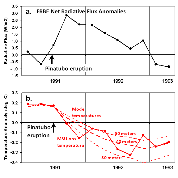
As can be seen in panel b, the MSU-observed temperature variations are consistent with a heat capacity equivalent to an ocean mixed layer depth of about 40 meters.

So, What is the Climate Model’s Sensitivity, Roy?
I think this is where confusion usually enters the picture. In running the above model, note that it was not necessary to assume a value for lambda, the net feedback parameter. In other words, the above model simulation did not depend upon climate sensitivity at all!

Again, I will emphasize: Modeling the observed temperature response of the climate system based only upon ERBE-measured radiative imbalances does not require any assumption regarding climate sensitivity. All we need to know was how much extra radiant energy the Earth was losing [or gaining], which is what the ERBE measurements represent.

Conceptually, the global-average ERBE-measured radiative imbalances measured after the Pinatubo eruption are some combination of (1) radiative forcing from the Pinatubo aerosols, and (2) net radiative feedback upon the resulting temperature changes opposing the temperature changes resulting from that forcing– but we do not know how much of each. There are an infinite number of combinations of forcing and feedback that would be able to explain the satellite observations.

Nevertheless, we do know ONE difference in how forcing and feedback are expressed over time: Temperature changes lag the radiative forcing, but radiative feedback is simultaneous with temperature change.

What we need to separate the two is another source of information to sort out how much forcing versus feedback is involved, for instance something related to the time history of the radiative forcing from the volcanic aerosols. Otherwise, we can not use satellite measurements to determine net feedback in response to radiative forcing.

Fortunately, there is a totally independent satellite estimate of the radiative forcing from Pinatubo.

SAGE Estimates of the Pinatubo Aerosols
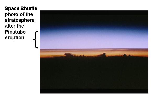
For anyone paying attention back then, the 1991 eruption of Pinatubo produced over one year of milky skies just before sunrise and just after sunset, as the sun lit up the stratospheric aerosols, composed mainly of sulfuric acid. The following photo was taken from the Space Shuttle during this time:
There are monthly stratospheric aerosol optical depth (tau) estimates archived at GISS, which during the Pinatubo period of time come from the SAGE (Stratospheric Aerosol and Gas Experiment). The following plot shows these monthly optical depth estimates for the same period of time we have been examining.
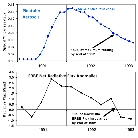
Note in the upper panel that the aerosols dissipated to about 50% of their peak concentration by the end of 1992, which is 18 months after the eruption. But look at the ERBE radiative imbalances in the bottom panel – the radiative imbalances at the end of 1992 are close to zero.

But how could the radiative imbalance of the Earth be close to zero at the end of 1992, when the aerosol optical depth is still at 50% of its peak?

The answer is that net radiative feedback is approximately canceling out the radiative forcing by the end of 1992. Persistent forcing of the climate system leads to a lagged – and growing – temperature response. Then, the larger the temperature response, the greater the radiative feedback which is opposing the radiative forcing as the system tries to restore equilibrium. (The climate system never actually reaches equilibrium, because it is always being perturbed by internal and external forcings…but, through feedback, it is always trying).

A Simple and Direct Feedback Estimate
Previous workers (e.g. Hansen et al., 2002) have calculated that the radiative forcing from the Pinatubo aerosols can be estimated directly from the aerosol optical depths measured by SAGE: the forcing in Watts per sq. meter is simply 21 times the optical depth.

Now we have sufficient information to estimate the net feedback. We simply subtract the SAGE-based estimates of Pinatubo radiative forcings from the ERBE net radiation variations (which are a sum of forcing and feedback), which should then yield radiative feedback estimates. We then compare those to the MSU lower tropospheric temperature variations to get an estimate of the feedback parameter, lambda. The data (after I have converted the SAGE monthly data to 72 day averages), looks like this:
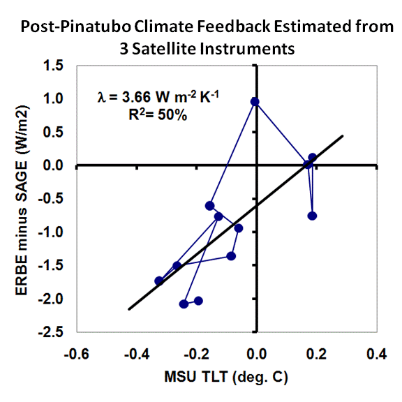
The slope of 3.66 Watts per sq. meter per degree corresponds to weakly negative net feedback. If this corresponded to the feedback operating in response to increasing carbon dioxide concentrations, then doubling of atmosphere CO2 (2XCO2) would cause only 1 deg. C of warming. This is below the 1.5 deg. C lower limit the IPCC is 90% sure the climate sensitivity will not be below.

The Time History of Forcing and Feedback from Pinatubo
It is useful to see what two different estimates of the Pinatubo forcing looks like: (1) the direct estimate from SAGE, and (2) an indirect estimate from ERBE minus the MSU-estimated feedbacks, using our estimate of lambda = 3.66 Watts per sq. meter per deg. C. This is shown in the next plot:
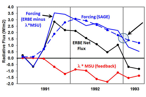
Note that at the end of 1992, the Pinatubo aerosol forcing, which has decreased to about 50% of its peak value, almost exactly offsets the feedback, which has grown in proportion to the temperature anomaly. This is why the ERBE-measured radiative imbalance is close to zero…radiative feedback is canceling out the radiative forcing.

The reason why the ‘indirect’ forcing estimate looks different from the more direct SAGE-deduced forcing in the above figure is because there are other, internally-generated radiative “forcings” in the climate system measured by ERBE, probably due to natural cloud variations. In contrast, SAGE is a limb occultation instrument, which measures the aerosol loading of the cloud-free stratosphere when the instrument looks at the sun just above the Earth’s limb.

Discussion
I have shown that Earth radiation budget measurements together with global average temperatures can not be used to infer climate sensitivity (net feedback) in response to radiative forcing of the climate system. The only exception would be from the difference between two equilibrium climate states involving radiative forcing that is instantaneously imposed, and then remains constant over time. Only in this instance is all of the radiative variability due to feedback, not forcing.

Unfortunately, even though this hypothetical case has formed the basis for many investigations of climate sensitivity, this exception never happens in the real climate system

In the real world, some additional information is required regarding the time history of the forcing — preferably the forcing history itself. Otherwise, there are an infinite number of combinations of forcing and feedback which can explain a given set of satellite measurements of radiative flux variations and global temperature variations.

I currently believe the above methodology, or something similar, is the most direct way to estimate net feedback from satellite measurements of the climate system as it responds to a radiative forcing event like the Pinatubo eruption. The method is not new, as it is basically the same one used by Forster and Taylor (2006 J. of Climate) to estimate feedbacks in the IPCC AR4 climate models. Forster and Taylor took the global radiative imbalances the models produced over time (analogous to our ERBE measurements of the Earth), subtracted the radiative forcings that were imposed upon the models (usually increasing CO2), and then compared the resulting radiative feedback estimates to the corresponding temperature variations, just as I did in the scatter diagram above.

All I have done is apply the same methodology to the Pinatubo event. In fact, Forster and Gregory (also 2006 J. Climate) performed a similar analysis of the Pinatubo period, but for some reason got a feedback estimate closer to the IPCC climate models. I am using tropospheric temperatures, rather than surface temperatures as they did, but the 30+ year satellite record shows that year-to-year variations in tropospheric temperatures are larger than the surface temperatures variations. This means the feedback parameter estimated here (3.66) would be even larger if scaled to surface temperature. So, other than the fact that the ERBE data have relatively recently been recalibrated, I do not know why their results should differ so much from my results.

WeatherShop.com Gifts, gadgets, weather stations, software and more...click here!


32 Responses to “Revisiting the Pinatubo Eruption as a Test of Climate Sensitivity”

Toggle Trackbacks

  1. peeke says:

    “The slope of 3.66 Watts per sq. meter per degree corresponds to weakly negative net feedback. If this corresponded to the feedback operating in response to increasing carbon dioxide concentrations, then doubling of atmosphere CO2 (2XCO2) would cause only 1 deg. C of warming. This is below the 1.5 deg. C lower limit the IPCC is 90% sure the climate sensitivity will not be below.”

    I think it would be very interesting if another event like this would produce the same resulting feedback.

  2. Eli Rabett says:

    You almost certainly should not use the MSU anomaly as a measure of the total effect of the eruption at the surface since the gaseous and aerosol products were distributed throughout the troposphere and into the stratosphere (changing over time) and that will affect the radiative balance. Whatever the result, the interpretation ain’t gonna be simple.

    OTOH, the MSU tropospheric and stratospheric anomalies, AFAEK, have never been used to interpret the effect of the distribution of gaseous and aerosol products and if they have not, it would be interesting to do so.

  3. Dan Kirk-Davidoff says:

    Hi Roy,

    This is pretty well-tilled ground.
    Have you read Douglass and Knox (2005), and Alan Robock’s response to them (2005); Doublass et al, 2006, and Boer et al., 2007, “Inferring climate sensitivity from volcanic events”?

    An important point addressed by these papers that you didn’t cover is the flux of heat from the deep ocean into the mixed layer. By 1993, the mixed layer has cooled by over half a degree- you could expect some heat flux upwards from the deep ocean (or, equivalently, a reduction of heat flux downwards) to result. Accounting for this would reduce the net forcing, and increase the estimate of sensitivity.

    Mixed layer models necessarily get too small a climate sensitivity because they can’t account for this: see figure 4 of Boer et al. (2007).

    Boer et al.’s conclusion is
    “The basic conclusion is that it is possible to obtain an
    estimate of the equilibrium climate sensitivity of the
    system from observations of strong volcanic events to
    within about 10% of the equilibrium value but that this
    requires that the forcing, the change in heat storage in
    the ocean and the temperature response all be known
    to high accuracy.”

    We didn’t have sufficient measurement of heat stoage in 1993 to do this, I would think we’ll be able to do a pretty decent job for the next Pinatubo-sized event.

    Cheers, Dan

    • Anonymous says:

      I am not a climate researcher but in chemical science and engineering so my questions may be irrelevant.

      Shouldn’t the deep ocean be a feedback rather than a forcing in this context? And shouldn’t such a feedback be negative resulting in a decrease of the climate sensitivity?

      When a radiative forcing increases the air temperature we obtain various feedbacks. One is that the outgoing long wave radiation increases according to the Stefan-Bolzmann equation, this is the negative Planck feedback. But also the heat transfer from the mixed layer to the deep ocean increases and this is a negative feedback just as the Planck feedback and should decrease the climate sensitivity since it decreases the temperature increase.

      My suggestion is that Dr. Spencer’s treatment in fact includes this negative feedback in the lambda value since any deep ocean feedback would diminish the temperature decrease caused by the Pinatubo aerosols resulting in a higher value of the feedback parameter lambda.

      • Anonymous says:

        Well, this question gets a little bit into the details of terminology. We’d prefer to think of feedbacks as phenomena that can influence the equilibrium solution, while the heat flux from the deep ocean to the mixed layer only moves heat around within the oceans. Of course, if the ocean circulation changes in response to a climate forcing, you could wind up changing the equilibrium solution, and then ocean effects would indeed be a feedback. The volcanic forcing case never lets the system get fully into equilibrium, so the distinction is a little murky.

        The main point is that we’re trying to estimate, from a sudden, brief volcanic event, the sensitivity of the system to a more gradual, sustained increase in CO2. Because the ocean is likely to behave differently in those two events, one needs to understand its behavior in some detail to be able to properly use information from the volcano “experiment” to predict the response to the CO2 “experiment.” There’s an important asymmetry between the two forcings: a short sharp cooling tends to make mixed layer cooler and more dense, and makes mixing with the deep ocean easier. A gradual warming, on the other hand, tends to make the mixed layer less dense, and thus to isolate the mixed layer from the deep ocean and reduce mixing. The Boer et al. paper does a nice job discussing these points.

        • Anonymous says:

          Thank you for your reply, Dr. Kirk-Davidoff.

          However, to me your arguments seem to support rather than contradict Dr. Spencer’s calculations resulting in a low climate sensitivity. An analysis using a simple conceptual heat transfer model suggests that such a low climate sensitivity may well be consistent with your arguments. The conceptual model is:

          (Heat flux from the mixed layer to the deep ocean) = (Transfer coefficient) * (Driving force) = (Transfer coefficient) * (Temperature difference between the mixed layer and the deep ocean)

          When the temperature of the mixed layer increases due to radiative forcing this heat flux increases due to increased driving force, diminishing the temperature increase When the temperature of the mixed layer decreases due to radiative forcing this heat flux decreases, diminishing the temperature decrease. Hence this heat flux represents a negative feedback.

          In the case of the Pinatubo aerosols this negative feedback wasn’t only influenced by the change in the driving force but the transfer coefficient also increased due to the abrupt density changes that you describe in your reply. This obviously decreased the negative feedback and lowered the lambda value.

          In the case of a gradual increase of the greenhouse gases the transfer coefficient was again influenced by density changes but this time the coefficient decreased. Again this obviously decreased the negative feedback and lowered the lambda value.

          Hence, Dr. Spencer has obtained a lambda value from the Pinatubo eruption that was lowered by the change in the transfer coefficient. This makes his lambda value to fit better with the lambda value for the gradual increase of greenhouse gases, since this latter lambda value also was lowered by the change in the transfer coefficient.

          Furthermore, in the Pinatubo case with its abrupt temperature change, the lambda value may well have been lowered more than in the greenhouse gas case with a more gradual temperature change.

          Hence, Dr. Spencers lambda value from the Pinatubo eruption may well be too low suggesting that the climate sensitivity could be even lower than according to his result.

          Pehr Bjornbom

          • Anonymous says:

            Hi Pehr,

            Here’s the situation. Over the vast majority of the surface area of the ocean, there is a shallow mixed layer (about 50 m in the tropics and varying from about 20 m in summer to about 100 m in winter in the extra-tropics, see: de Boyer Montιgut, C., G. Madec, A. S. Fischer, A. Lazar, and D. Iudicone (2004), Mixed layer depth over the global ocean: An examination of profile data and a profile-based climatology, J. Geophys. Res., 109, C12003, doi:10.1029/2004JC002378 )

            This sits on top of the thermocline, a region of several hundred meters where the temperature falls down to near 0°C.

            Cooling the mixed layer tends to deepen it, effectively mixing heat up from the thermocline, and making the effective heat capacity of the ocean larger. Warming the mixed layer tends to increase the buoyancy difference between the thermocline and the mixed layer, and making the thermocline shallower, reducing the effective heat capacity of the ocean. This happens each year (thus the shallower mixed layer in summer and deeper mixed layer in winter mentioned above).

            Now, this is all really a side point. Dr. Spencer has not taken into account *any* mixing of heat from the thermocline into the mixed layer in response to the Pinatubo cooling. In an equilibrium climate there is no global mean net heat flux between the the mixed layer and the thermocline, so to get an equilibrium climate sensitivity, you need to account for the transient flux of heat between these ocean layers, and subtract it from radiative forcing to which the boundary layer is responding.

            When you account for this, it turns out that a significant fraction of the heat that Dr. Spencer is assuming to flow out of the mixed layer (and causing it to cool) is actually flowing out of the deep ocean (See for example: Stenchikov, G., T. L. Delworth, V. Ramaswamy, R. J. Stouffer, A. Wittenberg, and F. Zeng (2009), Volcanic signals in oceans, J. Geophys. Res., 114, D16104, doi:10.1029/2008JD011673.) Thus the temperature change is larger in relation to the true forcing than what Dr. Spencer assumes.

            I’m speculating that because of the asymmetry of mixed layer warming and cooling, that if you compared a Pinatubo-type event with an “anti-Pinatubo” warming of the same magnitude, you’d get a larger response to the warming event than to the cooling event, but in either case, the response would be reduced by the flow of heat between the mixed layer and the thermocline, and it’s important not to assume that to be zero.

  4. Andrew says:

    The recovery from volcanic eruptions appears to be very rapid in the observed record. This would tend to suggest a relatively low sensitivity, but of course relative to what depends on the rate of heat mixing into the ocean. Still, models tend to predict much slower responses than indicated by volcanic eruptions, and several papers actually claim that the effect of Krakatoa (!) should still be present in the ocean! This is clearly not reasonable.

    By the way, with regard to Douglass and Knox, mentioned by Dr. Davidoff above, “Application of a dynamical two-box surface-atmosphere model to the Mount Pinatubo cooling event” by Robert Knox and Kevin LaTourette available on arxiv dot org, is an interesting extension of Knox’s earlier work with David Douglass.

    • Anonymous says:

      Hi Andrew,

      What did you think was interesting about the Knox and LaTourette (2008) paper?

      As far as I can see, they don’t make any progress on handling the interaction of the mixed layer and the ocean, and they don’t give any thought to the problem of the reaction time over land versus that over sea. They don’t even cite, let along respond to the numerous GCM studies which provide a substantially better fit to the data than the single layer models (e.g. Soden et al. 2002). They added a separate box for the atmosphere, but since, as Roy points out the atmosphere is pretty tightly coupled to the surface on time scales longer than a month or so, I’m not sure how much that adds to their analysis.

      Dan

  5. MapleLeaf says:

    Dr. Rabett says “You almost certainly should not use the MSU anomaly as a measure of the total effect of the eruption”

    I could have this wrong, but that wouldn’t that fact alone suggest that the above finding of transient climate response is not correct? I say TCR and not equilibrium climate sensitivity, but please do correct me if I also have that wrong. Thank you.

    • On what basis would he say such a thing? This is an issue I have studied more than anyone else. It turns out that the radiative feedback is much more highly correlated with tropospheric temperature than surface temperature at these time scales — with a peak corrrelation at zero days time lag!. This is something we demonstrate in our new JGR paper….(which will hopefully appear sometime this century). Then, since the TLT anomalies average about 1.2 x the surface temperature anomalies (30 years of 3 month average anomalies), you can then multiply the LT-based feedback parameter by another 1.2 to reference to the surface, which is the traditional reference for feedbacks.

      • Eli Rabett says:

        Given that the heat capacity of the surface is lots bigger than the heat capacity of the atmosphere, it is not surprising. Still, in this case you have to handle the fact that using the MSU you are making the measurement in the middle of the system and not at the bottom.

  6. Andrew says:

    Dr Davidoff,

    I did not in the least mean to imply that the paper was revolutionary! It is merely interesting, in that it elaborates on the physical issues involved.

    At any rate, it appears it is pretty trivial to get a decent fit to the eruption. I’m not surprised that more complicated models can improve the fits, although I’ll have to look into the paper you reference to see just how “substantial” an improvement the GCM’s result in.

  7. Steve Fitzpatrick says:

    Dan Kirk-Davidoff,

    Yup, if there is another Pinatubo sized volcano, ARGO data should produce a reasonably tight constraint on credible climate sensitivities in short order.

    Absent a major volcano, generating a reasonable constraint on climate sensitivity may take 10 years or more of accurate ocean heat content versus surface temperature changes.

    Either way, there may be a glimmer of light at the end of the “What is the real climate sensitivity?” tunnel. And none too soon as far as I am concerned.

  8. Your blog is very nice,thanks

  9. Pehr Bjornbom says:

    Hi Dan Kirk-Davidoff,

    Note that Dr. Spencer calculated the feedback parameter directly from observed data for radiation fluxes and for temperature using the following equation for the radiation fluxes:

    (Increase in outgoing radiation) = (Increase in outgoing shortwave radiation) + (Increase in outgoing longwave radiation) = – (Radiative forcing) + (Radiative feedback)*(Temperature anomaly)

    or

    – DeltaOR = Forcing_R – Lambda_R*T

    He obtained the DeltaOR from ERBE, the Forcing_R from the Pinatubo aerosol optical density and T from MSU temperature data. By plotting DeltaOR + Forcing_R versus T, Lambda_R is calculated as the slope of the fitted straight line. See the fourth figure in Dr. Spencer’s post.

    Lambda_R may also be calculated by fitting DeltaOR – Lambda_R*T to – Forcing_R as demonstrated in the fifth figure.

    Note that it’s essential to use the measured temperature anomalies in these calculations because the outgoing longwave radiation flux depends on the real, not a corrected, temperature.

    You are right in that the Lambda_R value doesn’t include the feedback effect of the deep ocean on the temperature of the mixed layer, since that feedback consists of heat exchange between the deep ocean and the mixed layer. However, this is a negative feedback which should increase the total Lambda value in the energy balance for the planet as given in the post:

    Lambda = Lambda_R + Lambda_DO

    where the value for the deep ocean feedback Lambda_DO > 0.

    Hence Lambda > Lambda_R = 3.66 W/m2/K.

    Consequently Dr. Spencer has calculated a lower limit of the Lambda value and consequently an upper limit of the climate sensitivity of around 1 K.

    Cheers, Pehr Bjornbom

  10. At the time Pinutubo errupted, the ocean was gaining energy from a solar/diminished cloud forcing of around 4W/m^2. I calculated this from the extra energy required to account for the steric component of sea level rise between 1993 and 2003. This would offset to a large extant the ~-3 to-5W/m^2 diminished insolation Pinutubo might have caused, leaving the ocean heat content little changed. The ~0.4C drop in SST around the time was no doubt partly caused by Pinutubo, but the ocean surface temp would have been on a downswing following the previous el nino anyway.

    If another Pinutubo occurred tomorrow, there would be a bigger negative effect on OHC, since the sun is quiet at the moment, and heat is leaving the ocean, rather than mixing down into it.

  11. Dan Kirk-Davidoff says:

    Hi Pehr,

    Okay, I started posting a little hastily there, and got distracted by the plot about diagnosing heat capacity.

    My comments above have to do with the problem of modeling the mixed-layer response to Pinatubo over time. If you don’t include mixed-layer/thermocline interactions, it looks like the temperature response is small due to an excessively sensitivity, when the real issue is that there’s extra heat flowing into the mixed layer (or equivalently, less heat flowing out) from the thermocline. It doesn’t make sense to think of the ocean mixed-layer/thermocline interaction as a feedback, because it’s zero in equilibrium in the global mean.

    As far as the effort to derive lambda directly from the difference between the SAGE forcing and ERBE, I’d argue that the very large unforced fluctuations of the net radiative balance make regression against a short temperature time series fraught with error. In this particular case, the difference between Dr. Spencer’s results and those of Forster and Gregory (2006) appear to be due to the fact that in the Pinatubo case, the GISS temperature excursion in late 1992 is substantially larger than the MSU excursion, which doesn’t peak until early 1993. Also the GISS temperature returns to near or above normal conditions in early 1993, which tends to flatten the regression line.

    • OK, this I must respond to. Dan, Pinatubo provided the single largest radiative forcing event in the satellite record, which means it’s radiative feedback signature will also be correspondingly large (in proportion to the temperature anomaly). The fact that we actually have a radiative forcing estimate for this event (from SAGE) means that we have the unusual opportunity to isolate a large feedback, in as direct a manner as possible. I’m finishing up a paper now for submission with the latest results, and the feedback component — between pre-Pinatubo and peak cooling post-Pinatubo — is over 2.5 Watts. If we cannot diagnose a feedback parameter from this event, we sure won’t be able to from any other event in the satellite record.

  12. Pehr Bjornbom says:

    It’s puzzling that Forster and Gregory got such a low Lambda value as 2.3 W/m2/K if they used GISS temperature anomalies. I have made a calculation using GISS by fitting ERBE – Lambda*T to SAGE. I found

    Lambda = 5.0 W/m2/K for GISS temperature data (climate sensitivity = 0.74 K/CO2-doubling).

    I simply minimized the sum of squares by trial and error, which easily can be done in a few minutes using an ordinary calculation sheet (Open Office Calc, for example).

    I read the ERBE and the SAGE data points from Dr. Spencer’s diagrams. However, I used a slightly different procedure for the temperature anomaly data points.

    Monthly average temperature anomalies were used and smoothed by applying B-splines with a data point order of ten (simply because this is available in Open Office Calc). The temperature points were then read from the smoothed curve and normalized by setting the anomaly to zero at 1991.1 years.

    Using this procedure with the UAH MSU monthly average temperature anomalies gave Lambda = 3.4 W/m2/K, the same that Dr. Spencer obtained within the limits of numerical error due to reading from diagrams etc.

    The same calculations using the HadCRUT3 and the NCDC NOAA monthly data gave Lambda values around 6 W/m2/K (climate sensitivity around 0.62 K/CO2-doubling).

    It’s interesting that the UAH MSU temperatures give a much better fit than the other three data bases. The sum of squares for the best fit was around twice as much for the latter data bases than for the UAH MSU one.

  13. Roger says:

    Any comments on this Science missive? “Observational and Model
    Evidence for Positive Low-Level Cloud Feedback
    Amy C. Clement,1* Robert Burgman,1 Joel R. Norris2

  14. Andrew says:

    Roy you have a heck of spam filter. I just linked to your post amount the Clement et al paper for this fellow, and apparently it ate that! Your own blog! Wow…I recommend some tweaking because that is too aggressive.

  15. Alexander Harvey says:

    Perhaps I am missing something, but I think there is a simpler way of putting things. Which avoids some confusion over the thermal nature of the land/oceanic/atmospheric system. I think that one simply does not worry about the heat storage term as it cancels out.

    Now:

    Cp*[dT/dt] = F – lambda*T

    is correct as stated, but all the arguments would work if it was put as:

    dE/dt = F – lambda*T

    {where E is the energy retained or stored by the system}

    This would be true no matter how the system was modelled, (slab ocean, upwelling- diffusive ocean, with or without atmospherice heat content, moisture, whatever).

    Now dE/dt is also what the combined (SW/LW) ERBE tries to measure so whatever the value of dE/dt one replaces it with the ERBE data. The energy balance combined (SW/LW) is just the rate of enrgy storage by the system, there is nowhere else for the heat to go if dE/dt is defined as rate of energy storage inside a system defined as everything below the altitude at which the ERBE tries to measure the balance.

    So one does not worry about the rate of heat storage per se; one balances the right hand side:

    F – lambda*T

    directly against the combined (SW/LW)ERBE data.

    What I am trying to say is that the method used gives the correct result; it does not need further corrections for oceanic heat uptake.

    This is to be contrasted to cases were ERBE data is not used and the heat balance has to be implied from a thermal model of the land/oceanic/atmospheric system or from OHC and a model of the land/atmospheric system, or some such methods.

    The line of argument used is insensitve to the exact nature of the processes behind dE/dt as this value does not appear in the final calculations.

    Now I may have this very wrong, but that is how it seems to me. It is I feel what gives the approach additional clarity. All that one needs to consider is whether F – lambda*T correlates strongly with the combined ERBE data, given ones choice of how to observe T.

    All that is being required of the model is the function F – lambda*T is a fair account of how the real world behaves, e.g. the real world reaction is linear in both F and T (including no time lag in the response).

    Alex

    • Anonymous says:

      I should have made it clear (e.g. replied to one of the posts that worried about the heat storage term) that I was not varying from Dr Spencer’s method, just trying to point out that the storage term is equal to the ERBE term and that it can be, and is simply replaced by the ERBE data.

      Alex

    • While it is true that the LHS of the equation can be rewritten in terms of heat content rather than temperature, if you assume no change in heat content, then there is no change in temperature, and thus no feedback to measure.

      • Anonymous says:

        Oh Dear!

        Thanks for the reply. Now I really am puzzled. I think the simplest way of clarifying is to ask whether you used the relationship

        ERBE = F – lambda*T to do your calculations (I apologies if I have the sign of ERBE wrong).

        If you do, the precise nature of the term represented by dE/dt (e.g. Cp*[dT/dt] or something accounting for more complicated response) is irrelevant.

        I think that your approach is insensitive to the nature of the thermal model (which is a big plus point).

        Why do I say a plus point? Because it is insensitive to arguments like:

        the lack of cooling in year 2 was due to an “El Nino” type of response being triggered.

        Now for that to hold one could not argue that extra heat that came from “somewhere” and that heat is significant ,as that does not impact the argument (or the equation).

        (That would still leave arguments of the form that sudden cooling gives a different value for Lambda to gentle warming; I make no such argument but someone could.)

        Personally, I think your argument could be put in stronger terms, in that is it is not subject to debate about heat storage/retention. The calculation of an effective depth is useful in the 40 metres is not unreasonable and adds creadence but is not central to the argument, as I see it.

        But to get back on track:

        Do you use:

        ERBE = F – lambda*T to do your calculations

        If so it is insensitive to a choice of a thermal model and hence a very strong line of argument.

        Now you say:

        “if you assume no change in heat content, then there is no change in temperature, and thus no feedback to measure.”

        What I am saying is that using ERBE makes the model WYSIWYG:

        If dE/dt = 0
        then ERBE = 0
        and F = lambda*T

        lambda = F/T

        Now that is not what happened, but the equation would still work if it had. By that I mean that the equation is formally correct irrespective of heat retention. If the system had no thermal mass dE/dt would indeed be zero but that would not imply that the temperature would not change, so I guess I do not understand your point:

        “if you assume no change in heat content, then there is no change in temperature, and thus no feedback to measure.”.

        Personally I think the approach is terrific, but for some reason I seem to think it is more terrific than you seem to do.

        But to clear things up, as I asked above:

        Do you drop the oceanic heat content term and set ERBE = F – lambda*T (as your diagrams indicate to me), if you do then I am not saying anything new just saying it louder.

        I hope I have been clear.

        Best Wishes

        Alex

  16. Pehr Bjornbom says:

    Here is a comment on the effect of the deep ocean on the value of the feedback parameter.

    Let us assume that the climate system consists of the troposphere and the mixed layer of the ocean. External to the climate system are the stratosphere and the deep ocean including the thermocline. We also neglect the effect of the land mass.

    Incoming power to this system is mainly the incoming solar radiation that is absorbed and not reflected = II_At S*dA W where II_At is the symbol for the double integral over the earth’s total surface area, At m2, and S W/m2 is the locally absorbed solar radiation.

    Outgoing from the climate system is the long-wave radiation = lambda_r *II_At (T_r – T_sp)*dA W where T_r is the temperature of the radiating layer in the atmosphere and T_sp is the temperature of the space (2.7 K). lambda_r W/m2/K is a transfer coefficient for radiative heat transfer and assumed constant.

    Outgoing is also the heat flow from the mixed ocean layer through the thermocline to the deep ocean = lambda_do*II_Ado (T_ml – T_do)*dA W where we integrate over the area between the mixed layer and the deep ocean. T_ml is the temperature of the mixed layer and T_do of the deep ocean. lambda_do W/m2/K is a transfer coefficient for convective heat transfer between the mixed layer and the deep ocean.

    Let us look at how the energy content of the climate system, E J, changes from a time zero when E = E0 J. Then
    dE/dt – dE0/dt = dE/dt = II_At (S-S0)*dA – lambda_r*II_At (T_r – T_r0)*dA – lambda_do*II_Ado (T_ml – T_ml0)*dA (1)

    This can be written as integral mean values (symbolized with _m) over the respective areas:
    dE/dt = (S-S0)_m*At – lambda_r*(T_r – T_r0)_m*At – lambda_do*(T_ml – T_ml0)*Ado (2)

    We now assume that the temperature anomalies are the same in the atmosphere and in the mixed layer (or alternatively that they are proportional):
    dE/dt = (S-S0)_m*At – (lambda_r*At + lambda_do*Ado)*(T – T0)_m (3)

    Let us apply this equation for the hypothetical case that we go from one so-called equilibrium state of the climate system to another. This means that we start from one steady state with the energy content E0 J, not varying with time, we perturb the system with a forcing Delta S W/m2 and await the new steady state with a constant energy content E J. At the new steady state dE/dt = 0 giving:

    (T – T0)_m = (S-S0)_m/(lambda_r + lambda_do*Ado/At) or Delta T = Delta S/lambda (4)

    The denominator in this equation is the feedback parameter and we can see that the deep ocean acts as a negative feedback decreasing the effect of the forcing in the numerator.

    Obviously the first two terms in equation (2) are measured by the ERBE. If the change in the forcing is known, as during the Pinatubo eruption, the radiative feedback parameter lambda_r can be determined by using the ERBE data and for example the UAH MSU temperature anomalies, as carried out by Dr. Spencer. This is done without having to use equation (2). However, what equations (2) and (4) tell us is that the total feedback parameter lambda is greater than lambda_r because of the negative feedback from the deep ocean.

  17. Mac says:

    Sorry to bother you again, I have left another post a few days ago but that seems to have been lost πŸ™

    Can you please comment on the similitudes and differences of your model and the one used by Stephen Schwartz in his 2007 paper linked below:

    http://www.ecd.bnl.gov/steve/pubs/HeatCapacity.pdf

    • As I recall, Schwartz tried to get climate feedbacks from the time scale of observed variability in ocean temperatures. It’s a different method, but I suspect the model was similar…I would have to go back and look.

  18. This piece of writing is really a nice one it helps new web users, who are wishing for blogging.

  19. You gave me even more new perspectives. Your post is very helpful to me. Thank you.

Leave a Reply