U.S. Temperature Update for May 2012: +1.26 deg. C

June 8th, 2012 by Roy W. Spencer, Ph. D.

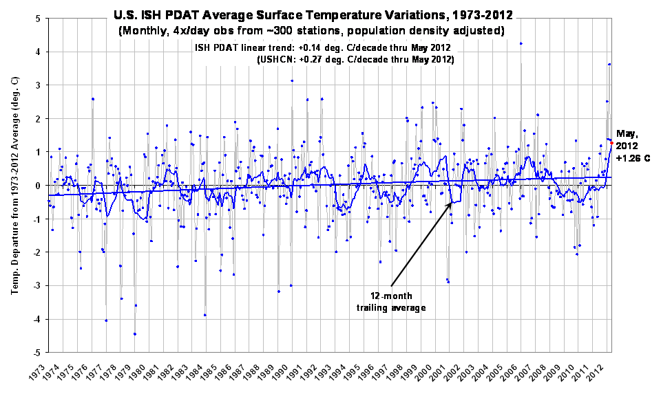
The U.S. lower-48 surface temperature anomaly from my population density-adjusted (PDAT) dataset was 1.26 deg. C above the 1973-2012 average for May 2012, with a 1973-2012 linear warming trend of +0.14 deg. C/decade (click for full-size version):
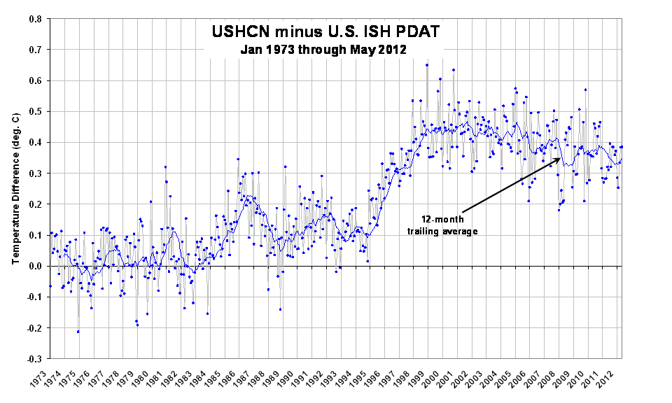
The corresponding USHCN anomaly computed relative to the same base period was +1.65 deg. C, with nearly double my warming trend (+0.27 deg. C/decade). The warming of the USHCN relative to my dataset shows that most of the discrepancy arises during the 1996-98 period:
Despite the weaker warming trend in my dataset, Spring 2012 still ranks as the warmest spring since the beginning of my record (1973). The 12-month period ending in May 2012 is also the warmest 12-month period in the record.

Due to a lack of station data and uncertainties regarding urban heat island (UHI) effects, I have no opinion on how the recent warmth compares to, say, the 1930s. There is also no guarantee that my method for UHI adjustment since 1973 has done a sufficient job of removing UHI effects. A short description of the final procedure I settled on for population density adjustment of the surface temperatures can be found here.


25 Responses to “U.S. Temperature Update for May 2012: +1.26 deg. C”

Toggle Trackbacks

  1. Nikolaj says:

    So, if I am not wrong the situation is as follows: the raw data 1973-2012 do not show any warming trend.
    Roy Spencer earlier: “Virtually all of the USHCN warming since 1973 appears to be the result of adjustments NOAA has made to the data, mainly in the 1995-97 timeframe.”

    However, when the dubious TOBS adjustments are applied you get the official figure of 0.27 C/decade. You NOW accept that adjustment as legitimate, but then decrease the trend by correcting for the population density. You are actually doing the downward adjustment of the previous upward adjustment by removing the half of the trend fabricated by the upward adjustment. You are not upset anymore that NOAA essentially fabricated the entire warming trend 1973-2012!!!

    And further, another strange fact. When warned that your earlier population density adjustment contradicted your UAH data for USA which show 0.22 C/decade of warming you said:

    Spencer 2: “The monthly correlation between the two datasets is 0.87, so there is reasonably good agreement on that time scale, but a time series plot of their difference suggests some sort of step jump in 1995:

    Now, 1995 happens to be when the NOAA-11 satellite was replaced by NOAA-14, and those two satellites had to be intercalibrated with NOAA-12, which was going through its own diurnal drift. So, there might be a diurnal drift issue here that has not been sufficiently accounted for. Maybe our new (but unfinished) diurnal adjustment strategy for Version 6 of the UAH dataset will shed light on this.”

    Strange, it seems that your “warming” trend started somehow in the same time as NOAA’s, in 1995. Or maybe this issue is not relevant anymore, since you happily found an adjustment procedure that would not make your data look so bad?

  2. I note you specify lower 48 states, can’t speak for them, but up here on the east shore of Superior we had one of the coolest May I can remember…

  3. Dan Pangburn says:

    The U.S. covers less than 2% of the earth’s surface. So . . . shrug.

  4. Harold Pierce Jr says:

    ATTN: Roy and All

    RE : How to Compute Weather Noise

    I outline a simple method for computing “weather noise” or variation in temperature at a station due to local weather.

    1. Do multi-decadal analyses for Tmax and Tmin for several

    days of the of the year. I use the eqinoxes and the

    soltices.

    2. For each decadal interval compute the classical average

    deviation from the mean for Tmax and Tmin.

    3. The formula weather noise(WN)is: WN = AD – RT, where AD

    is the average deviation and RT is resolution of the

    thermometer which is typically 0.1 deg.

    Since sunlight is constant over the sample interval, the variation of local temperature is due to events suchas as clouds with or without rain, snow, fog, wind, changes in air pressure, etc.

    I did these calculations from temperature data from the weather station at Qusinto, B.C. for the sample period 1895-2009 and got WN = 1.4 deg C for Tmax and T min.

    For China Lake WN = 0 deg C for Tmax and Tmin. The sample period was 1945-2009.

    The calculations should carried out for each day of the year
    because there could be seasonal effects in the temperate zones. For example in summer the are long periods of sunny dry days whereas in winter there is more varible weather.

    Suppose we do these calculation from temp data from many _rural_weather stations and get WN = 1 deg C for Tmax and Tmin.

    The climate scientists would no longer be able to claim there is global warming since the mean global temp anomaly
    from 1900 to present is on ca. 0.8 deg.

  5. Loren Marz says:

    I’m a CCM and recently-retired operational meteorologist for the National Weather Service.

    I’m sure this has been discussed previously, but can someone briefly explain why there are not + or – 1 degree C error bars around all U.S. temperature data points? I know for a fact the the temp instrument error on the ASOS (Automated Surface Observation System) sites is + or – 1.8 degrees F (+ or – 1 degree C).

    I have always been highly skeptical of climate model results based on my experience with Numerical Weather Prediction (NWP) models. NWPs have essentially no skill at 7 days, never mind decades in the future.

    I’m also not sure how IPCC can conclude a 0.74 degree C increase in global temps in the past 150 years when that increase is within the margin-of-error of the current instrumentation.

    Can someone enlighten me on this conundrum?

  6. Andrew says:

    Loren Marz- A few groups do report uncertainty estimates, although they are rarely plotted.

    Some questions for you about the ASOS uncertainty: is it the estimate of the absolute error, or the estimate of the time varying random error? The absolute error is not important for temperature change, but the time varying random error would be.

    Even so, if you have a very large number of stations, one would expect random errors to largely cancel out.

  7. Nigel Harris says:

    The issue of how you can detect a change in average temperature that is smaller than the measurement error of an individual thermometer is something I see a lot in comments on these sites. If you measure temperatures at several thousand sites (using several thousand different thermometers) then you can determine the average temperature to a much greater precision than an individual thermometer. As long the errors are random rather than systematic (that is, some thermometer readings are high, others are low) then they don’t exactly “largely cancel each other out”, but the cumulative error of the total of all thermometer readings grows as the square root of the number of thermometers, rather than linerarly. So when you divide that total by the number of thermometers to get the average temperature, the error bars can be far narrower than the error on an individual thermometer.

    If the error on each thermometer is +/- 1C, then with 100 thermometers, the error on the average temperature is only +/- 0.1C, and with 10,000 thermometers it is +/- 0.01C.

    If you had a weight loss class of 100 people, and scales that measured their weight the nearest 5 pounds, you might think it hopeless to be able to detect any change in average weight of the group of less than 5 pounds. But it is not so. If you add up all the weights of the 100 people, the error on the total is very unlikely to exceed 50 pounds. So the average can be known with a precision of less than one pound. If you measure everybody’s weight again two weeks later, an average loss of just one pound will be easily detectable. And that’s with only 100 measurements. Global temperature datasets are based on thousands of measurements.

  8. Joseph says:

    “Global temperature datasets are based on thousands of measurements.”

    I don’t know if Nigel Harris is refering to the number of data points in a single thermometer dataset or the total number of thermometers used in creating the global temperature. It really doesn’t matter since they are both far short of being thousands. Since temperature readings are only used from the first day of the month only records that are complete for 84 years have even one thousand datapoints. Most are missing points here and there and few go so far back. The number of thermometers taking tempueratures worldwide is large, but less then 200 are actually used in calculating the global temperature.

  9. Loren Marz says:

    OK, thanks. I assumed there must be a logical explanation; I’ve just never seen it explained.

    Now that you mention it, I vaguely recall that statistical theory (please forgive me…it’s been a L-O-N-G time since I took a statistic course).

  10. Harold Pierce Jr says:

    The reason there are no error given for temp measuremnts is that this not necessary for everyday weather reports to the public. Weather stations were not designed for use by research scientists.

    The reason there was once a vast network of weather stations was to provide weather data to the local area for practical reason. Farmers want to know temperatue and important info such as degree days and local weather to schedule for example harvesting of crops such cereal grains.

    Typically, local weather data was broadcast locally by radio or was available from the Ag ext service.

    Highway maintence guys want to if there is freezing temperature and snow is in the local forecast so they can get the trucks ready for salting and sanding. For them, the important temperature is 32 deg F.

    Utilites use local temperature data to estimate the electricity required, but they only need temp data to the nearest degree.

    The reason you see the clim scientist making a big deal about 0.1 deg is that they have never had a course in intrumental analysis which is an upper division course for chem and physics majors and engineers.

    I have modern text on meterology and there is no info on the practical aspects of temp measurements.

    Today most weather stations are at airports because pilots need to local weather conditions which is important for safe takeoffs and landings.

  11. Brian D says:

    Dr. Spencer, what happened to the interactive temp graph on your Discover site?

  12. Emily says:

    Some field work was done to check the accuracy of temp stations around the country– surfacestations.org
    It all publicly available information including a photo database and weather station metadata. I recommend checking it out.

  13. Frank says:

    This is an average for the lower 48, right? If that’s the case, how do below normal temps for the Pacific Northwest factor into this national average? (For instance, June in Seattle is so far three degrees below normal and May was 0.7 degrees below normal.)

    Does that mean many places were far warmer than normal? Why has the PNW been cooling for the last six years while the rest of the country seems to be warming?

  14. Dale Hill says:

    I have been following the global AMSU-A Temperatures for a while and have been wondering why there is an annual variation of about 2 degrees between July and December/January. Is there a simple explanation?

    • Massimo PORZIO says:

      Yes, I guess it is the different land/sea ratio between the Northern and the Southern hemisphere.
      Sea water has longer thermal time constant than land.

    • RW says:

      Dale,

      Actually, it’s mostly related to perhelion/aphelion cycle and changes in the albedo throughout the year. Since perhelion in January coincides when the albedo is at its maximum, it’s about 3C cooler instead of 3C warmer in January on global average.

      What no one seems to be able to explain is how can the oceans supposedly take decades to respond changes in forcing, like from 2xCO2, if the Earth’s global average temperature changes by 3C in just 6 months time? This much change this fast doesn’t support anywhere near that long of a response time to changes in incident energy.

      • Dale says:

        RW,
        Thank you for the additional clarification. I was wondering about orbital effects as well. It is interesting that the albedo trumps the perihelion so strongly.

        • RW says:

          What matters is how much of the Sun’s energy enters the system, which is of course is ultimately determined by the albedo. It just so happens that at this point in time, perihelion in January coincides with maximum reflectivity due to the ice and snow accumulation in the Northern Hemisphere winter.

  15. Dan Pangburn says:

    A thermal analysis reveals that the effective thermal capacitance of the oceans is about 30 times everything else.

    This slows the ongoing temperature decline trend to about -0.1C per decade. This decline is in spite of the continued rising level of atmospheric carbon dioxide.

  16. iya says:

    @RW and Dan Pangburn
    I’ve never seen a convincing argument in favor of a decade or even longer “pipeline”, either.

    The time constant of the atmosphere and ocean is a few days and months respectively. The deep ocean is practically isolated from the surface, almost like the Earth core. If it filled with the dense Mediterranean water, it would reach 13°C, irrespective of CO? and without influencing the surface temperatures.
    Just to clarify, I’m not talking about natural cycles like ENSO, PDO and AMO; these can and do mask a potential global warming signal, I’m saying a warmer ocean doesn’t matter (in contrast to a warmer atmosphere, which determines the outgoing radiation) and its coupling is so low that it does not even slow down any surface warming or cooling significantly.

    • Massimo PORZIO says:

      @iya & RW
      My one was just a guess, reading your explanation convinced me that you are right.

      Does anybody knows which is the effective reflection coefficient of the sea water for the whole hemispheric area?
      I mean: by night you can see reflected on the sea the Moon and the stars almost the same as you see them directly (I know our eyes have a little dynamics, please well weight my “almost the same” statement); since the rays in this case remains parallels each other and typically the field of view of a radiometer is little, the measured reflected intensity may highly varies by the angle between the source (the Sun) and the observer (the radiometer) on the reflection layer (the spheric surface).
      My question is: how do we measure the outgoing visible radiation to the outer space?

  17. Nige Cook says:

    The false idea that H2O has a purely positive feedback, amplifying the warming due to CO2, was put forward in 1896 by Stockholm’s famous chemist Svante Arrhenius (inventor of the famous exponential reaction rate equation, showing the influence of variables like temperature on chemical reactions), according to Dr Spencer R. Weart’s book, “The Discovery of Global Warming”, Harvard University Press, 2003, page 5.

    Arrhenius argued that increasing CO2 in the atmosphere causes a “positive feedback” from H2O simply because CO2 it warms the atmosphere, and warmer air can hold more moisture. The extra water vapour, H2O, in the atmosphere then amplifies the trivial direct effect of the CO2 increase, producing a substantial temperature rise.

    Arrhenius ignored the cloud cover problem: the more water vapour that evaporates, the more cloud cover (an effect that can’t occur inside a politically convenient glass-ceiling “greenhouse effect” propaganda model). Also, if water vapour had a purely positive feedback, Earth’s oceans would have boiled away long ago in a runaway greenhouse effect. There must therefore be some reversal of positive H2O feedback to negative HO2 feedback as the temperature rises, or we wouldn’t exist in the first place.

    There are data that seem to validate Calder (the former 1960s editor of New Scientist, who takes the opposite view to today’s magazine), who correlates the “Wilson cloud chamber” effect of nuclear physics (cirrus cloud cover at circa 15,000 feet altitude) with cosmic rays which form condensation trails to start cloud formation: http://calderup.wordpress.com/2012/03/03/climate-physics-101/

    Extending this Wilson cloud chamber mechanism for cloud cover to cause climate change, Calder points out in a more recent post that galactic cosmic rays from nearby supernovas peaked 250 million years ago, when the Permian period ended (mass extinctions).

    One other thing to point out is that the tree-ring and ice core oxygen ratio temperature proxies that show relatively little climate change (the handle of the hockey stick) before 1900, implicitly assume that cloud cover remains constant. Because tree growth and water evaporation depend on sunlight energy (not just air temperature), cloud cover exerts an effect. If cloud cover increases in hot periods due to water evaporation, it cancels out much of the variation in tree ring growth (and the preferential sublimation of light oxygen isotopes in ice cores) that would otherwise occur. This is why the hockey stick handle is a horizontal line with little vertical variation: the false assumption that cloud cover is constant (independent of temperature) leads to an underestimate the true temperature variations that occurred.

    The reality seems to be that the climate is not as stable as the IPCC proxies claim: all the proxies suffer the same delusion of constant cloud cover. This makes them all underestimate natural climate variability. The same error leads them to minimise attention on negative feedback from increasing cloud cover as temperature rises. The only risk they see is the risk of not taking action now to deal with their “Reichstagg Fire”. However, the costs of trying to regulate the climate pose big risks themselves in an economic depression.

  18. After reviewing the comments here We understand a lot more

Leave a Reply