Will Humanity Ever Reach 2XCO2? Possibly Not

February 1st, 2020 by Roy W. Spencer, Ph. D.

Summary

The Energy Information Agency (EIA) projects a growth in energy-based CO2 emissions of +0.6%/yr through 2050. But translating future emissions into atmospheric CO2 concentration requires a global carbon budget model, and we frequently accept the United Nations reliance on such models to tell us how much CO2 will be in the atmosphere for any given CO2 emissions scenario. Using a simple time-dependent CO2 budget model forced with yearly estimates of anthropogenic CO2 emissions and optimized to match Mauna Loa observations, I show that the EIA emissions projections translate into surprisingly low CO2 concentrations by 2050. In fact, assuming constant CO2 emissions after 2050, the atmospheric CO2 content eventually stabilizes at just under 2XCO2.

Introduction

I have always assumed that we are on track for a doubling of atmospheric CO2 (“2XCO2”), if not 3XCO2 or 4XCO2. After all, humanity’s CO2 emissions continue to increase, and even if they stop increasing, won’t atmospheric CO2 continue to rise?

It turns out, the answer is probably “no”.

The rate at which nature removes CO2 from the atmosphere, and what controls that rate, makes all the difference.

Even if we knew exactly what humanity’s future CO2 emissions were going to be, how much Mother Nature takes out of the atmosphere is seldom discussed or questioned. This is the domain of global carbon cycle models which we seldom hear about. We hear about the improbability of the RCP8.5 concentration scenario (which has gone from “business-as-usual”, to “worst case”, to “impossible”), but not much about how those CO2 concentrations were arrived at from CO2 emissions data.

So, I wanted to address the question, What is the best estimate of atmospheric CO2 concentrations through the end of this century, based upon the latest estimates of future CO2 emissions, and taking into account how much nature has been removing from the atmosphere?

As we produce more and more CO2, the amount of CO2 removed by various biological and geophysical processes also goes up. The history of best estimates of yearly anthropogenic CO2 emissions, combined with the observed rise of atmospheric CO2 at Mauna Loa, Hawaii, tells us a lot about how fast nature adjusts to more CO2.

As we shall see, it is entirely possible that even if we continued producing large quantities of CO2, those levels in the atmosphere might eventually stabilize.

In their most recent 2019 report, the U.S. Energy Information Agency (EIA) projects that energy-based emissions of CO2 will grow at 0.6% per year until 2050, which is what I will use to project future atmospheric CO2 concentrations. I will show what this emissions scenario translates into using a simple atmospheric CO2 budget model that has been calibrated with the Mauna Loa CO2 observations. And we will see that the resulting remaining amount of CO2 in the atmosphere is surprisingly low.

A Review of the CO2 Budget Model

I previously presented a simple time-dependent CO2 budget model of global atmospheric CO2 concentration that uses (1) yearly anthropogenic CO2 emissions, along with (2) the central assumption (supported by the Mauna Loa CO2 data) that nature removes CO2 from the atmosphere at a rate in direct proportion to how high atmospheric CO2 is above some natural level the system is trying to ‘relax’ to.

As described in my previous blog post, I also included an empirical El Nino/La Nina term since El Nino is associated with higher CO2 in the atmosphere, and La Nina produces lower concentrations. This captures the small year-to-year fluctuations in CO2 from ENSO activity, but has no impact on the long-term behavior of the model.

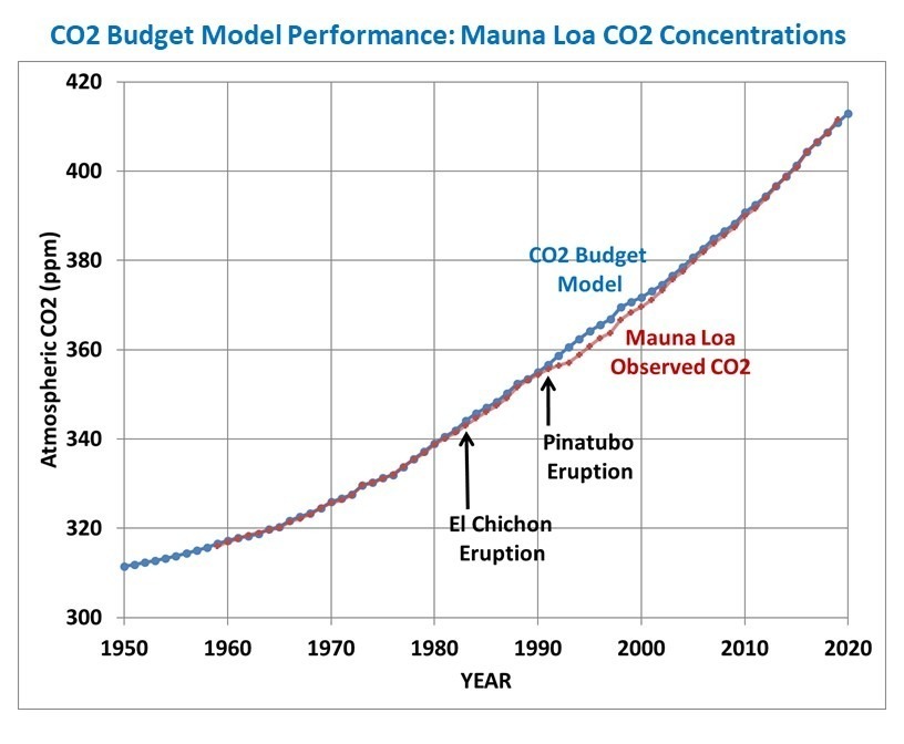
The model is initialized in 1750 with the Boden et al. (2017) estimates of year anthropogenic emissions, and produces an excellent fit to the Mauna Loa CO2 observations using the assumption of a baseline (background) CO2 level of 295 ppm and a natural removal rate of 2.33% per year of the atmospheric excess above that baseline.

Here is the resulting fit of the model to Mauna Loa data, with generally excellent results. (The post-Pinatubo reduction in atmospheric CO2 is believed to be due to increased photosynthesis due to an increase in diffuse sunlight penetration into forest canopies caused by the volcanic aerosols):

Fig. 1. Calibrated CO2 budget model compared to the Mauna Loa, Hawaii CO2 observations. The model is forced with the Boden et al. (2017) estimates of yearly anthropogenic CO2 emissions, and removes CO2 in proportion to the excess of atmospheric CO2 above a baseline value.

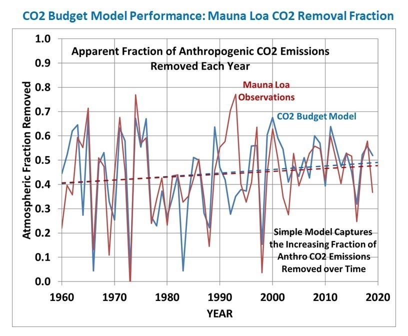
The model even captures the slowly increasing trend in the apparent yearly fractional removal of CO2 emissions.

Fig. 2. Yearly apparent fraction of anthropogenic emissions removed by nature, in the Mauna Loa observations (red) versus the model (blue).

Model Projections of Atmospheric CO2

I forced the CO2 model with the following two future scenario assumptions:

1) EIA assumption of 0.6% per year growth in emissions through 2050
2) Constant emissions from 2050 onward

The resulting CO2 concentrations are shown in Fig. 3, along with the UN/IPCC CO2 concentration scenarios, RCP2.6, RCP4.5, RCP6.0, and RCP8.5, used in the CMIP5 climate model projections.

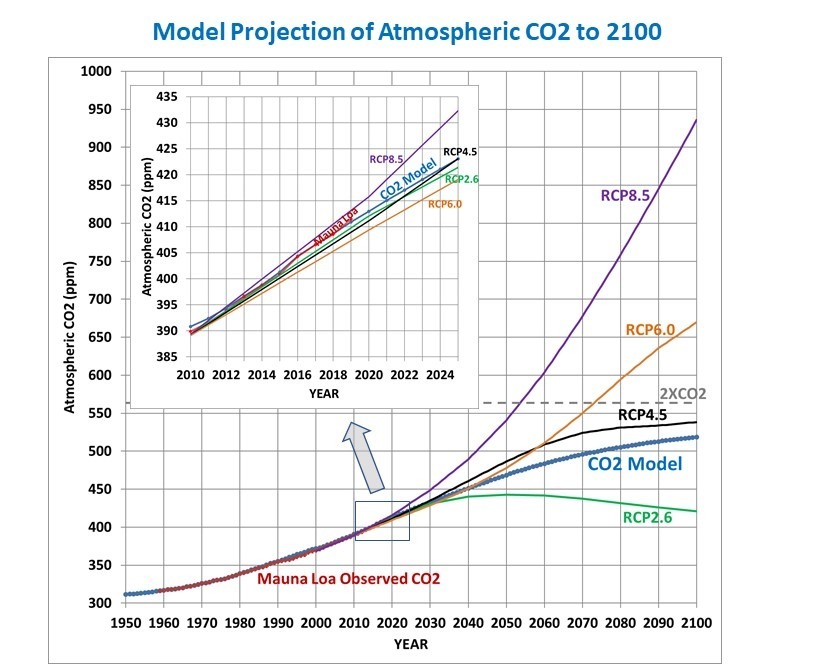
Interestingly, with these rather reasonable assumptions regarding CO2 emissions, the model does not even reach a doubling of atmospheric CO2, and reaches an equilibrium CO2 concentration of 541 ppm in the mid-2200s.

Discussion

In my experience, the main complaint about the current model will be that it is “too simple” and therefore probably incorrect. But I would ask the reader to examine how well the simple model assumptions explain 60 years of CO2 observations (Figs. 1 & 2).

Also, I would recall the faulty predictions many years ago by the global carbon cycle modelers that the Earth system could not handle so much atmospheric CO2, and that the fraction which is removed over time would start to decrease. As Fig. 2 (above) shows, that has not happened. Maybe when it comes to photosynthesis, more life begets still more life, leading to a slowly increasing ability of the biosphere to remove excess CO2 from the atmosphere.

Given the large uncertainties in how the global carbon cycle responds to more CO2 in the atmosphere, it is entirely reasonable to hypothesize that the rate at which the ocean and land removes CO2 from the atmosphere is simply proportional to how high the atmospheric concentration gets above some baseline value. This simple hypothesis does not necessarily imply that the processes controlling CO2 sources and sinks are also simple; only that the net global rate of removal of atmospheric CO2 can be parameterized in a very simple form.

The Mauna Loa CO2 data clearly supports that hypothesis (Fig. 1 and Fig. 2). And the result is that, given the latest projections of CO2 emissions, future CO2 concentrations will not only be well below the RCP8.5 scenario, but might not even be as high as RCP4.5, with atmospheric CO2 concentrations possibly not even reach a doubling (560 ppm) of estimated pre-Industrial levels (280 ppm) before leveling off. This result is even without future reductions in CO2 emissions, which is a possibility as new energy technologies become available.

I think this is at least as important an issue to discuss as the implausibility (impossibility?) of the RCP8.5 scenario. And it raises the question of just how good the carbon cycle models are that the UN IPCC depends upon to translate anthropogenic emissions to atmospheric CO2 observations.


355 Responses to “Will Humanity Ever Reach 2XCO2? Possibly Not”

Toggle Trackbacks

  1. spike55 says:

    Towards 700ppm https://i.postimg.cc/3xKD6YXS/Towards700.png

    We can get there.

    Come on, must try harder….

    • Chris Hanley says:

      Hear! hear!
      Assuming Dr Spencer’s assessment is valid, and I’m not qualified to judge, then it is a good test of the sincerity of ‘alarmists’.
      If they genuinely fear the supposed effects of human CO2 emissions they will be applauding.
      If they are simply using CO2 emissions as a political tool they will have trouble hiding their disappointment.

      • lewis b guignard says:

        RE: Chris Hanley,

        It has long been known that the alarmists are using CO2 emissions as a political tool. At this point there are a number of beneficiaries of the alarmist’s programs, but, generally, the people who will suffer the most are, to use HRC’s term, the deplorables.

        • Joseph Zorzin says:

          Here’s their agenda: https://ajustclimate.org/

          “a vision for an equitable and just climate future”

          “The Equitable and Just National Climate Platform advances the goals of economic, racial, climate, and environmental justice….”

    • Bob Weber says:

      We’ll never get it there, no matter how hard we try.

      Some facts should dispel any notion that MME (Boden etal) drives ML CO2. Real changes in ML CO2 are followed by MME changes by years of lag:

      https://i.postimg.cc/523gBrc9/Dep-Ave-Detr-Int-Ann-Change-CO2-MME-v-ML.png

      https://i.postimg.cc/ZR1xYtNH/Derivatives-and-Trends-of-MME-v-ML-CO2.png

      The assumptions underlying the head post model are wrong, and so is the model. Real adjusted for inflation CO2 is declining naturally (green line in the first plot), resulting from long-term changes to tropical temperatures, according to my all-natural CO2 model, of which MME is a tiny insignificant fraction:

      https://i.postimg.cc/gjsfgHXR/CO2-vs-30y-Nino-Intrayear-Ratio.jpg

      The last plot indicates CO2 is outgassed in perfect proportion to the Nino region temperature ratio of the first to the second half of the year (NIR), following natural and biological cycles and physical laws.

      Climate and changes never stopped being all-natural.

  2. Marc Facer says:

    The rate of annual increase in co2 = approx from memory 2.5 ppm – that trend rate increase is actually slowing – https://www.esrl.noaa.gov/gmd/ccgg/trends/gl_gr.html
    If the increase in co2 is actually due to humans (something that I see as a good thing)I feel with the actual increase of renewables will slow rates of increase futher & the natural increase in sinks will catch up more-
    Humans emit around 4.5 % of annual global co2 emissions – that is small by global standards & I would have thought that natural sinks would have accounted for most of that by now (they will always be catching up but)
    You hear about trees growing in certain places growing up to 75% faster (warmer environment – longer growing seasons increased co2) – and that the Earth is growing more trees & getting greener – thats certainly has to be increasing takeup significantly
    When you look at annual increase in co2 graphs such as what I posted – years such as 1991 & Mt Pinataubo erupting – the Earth cools and annual increase falls to nothing – that shows that much of it is natural as human output remains much the same each year
    I have much yet to learn but I cant accept that early scientific measurements such as those in the 1800’s were incorrect & I do not accept that co2 levels are constant – everything else in climate is cycles & the carbon budget is self controlling – for everything we produce nature will eventually sequester it

    • Roy W. Spencer says:

      Yes, I agree, I would wager there are natural cycles in CO2 content.

      • E. Swanson says:

        Dr. Spencer, One of those natural cycles is the THC sinking at polar latitudes. The THC process involves the yearly formation of sea-ice, during which brine is expelled, causing the surrounding water to become more dense than it would otherwise be. It is apparent that the location(s) for the sinking are limited and there’s evidence that the THC is already weakening. Since the very cold water which sinks carries more CO2 with it, if the THC slows, as many models have forecast, then that mode of CO2 removal will also be reduced.

        You noted that after the Pinatubo eruption, the rate of increase in CO2 slowed. It’s possible that this cooling temporarily increased the THC sinking with faster CO2 removal, a possibility which can not be assessed, since there isn’t much oceanographic data available from the period. Another possibility is that ocean biological productivity was reduced due to the reduction in sunlight reaching the surface. Do you have a reference to support your comment that Pinatubo’s effects were due to increased photosynthesis by land based plants?

      • Anon_Scientist says:

        Cosmic rays cause virtually all climate change by seeding clouds, not tasteless, colorless and odorless carbon dioxide gas comprising one molecule in 2,500 and, along with water vapor and methane, cooling all the other air molecules especially at night, radiating some of their energy back to Space.

        The temperature gradient in every planetary troposphere is formed by gravity in accord with the maximum entropy production associated with the Second Law of Thermodynamics. It is NOT caused by the radiating or absorbing properties of IR-active (“greenhouse”) gases and in fact they reduce the gradient and thus cool the surface. This is evident when comparing regions with varying concentrations of water vapor. If climatology “science” were correct, then rainforests could be shown (with their false physics) to be 50 to 80 degrees hotter than deserts. That is just how WRONG is the fictitious, fiddled physics of climatology.

        Circulate this message!

        • barry says:

          A Non-scientist

          Let’s play out your wondrous contention.

          We know for a fact that the temperature gradient is negative (gets colder) from the surface to the tropopause: from the tropoause to the stratopapuse the gradient is positive: from the tropoapuse to the mesopause the temperature gradient inverts again.

          If gravity determines temperature gradient, as you say, then we must conclude that gravity also inverts at each layer of the atmosphere. Jump out of a plane in the stratosphere and you should head spacewards until you reach the mesopause, where presumably you become trapped.

          With your ‘physics’ engineering a space elevator becomes a lot easier. If only your physics were true.

    • lewis b guignard says:

      As a side note: a ton of cellulose takes about 1000 lbs of C

  3. Dr. Roy, I wrote about this in my post below, and came to the same conclusion.

    w.

    https://wattsupwiththat.com/2017/01/24/apocalypse-cancelled-sorry-no-ticket-refunds/

  4. Entropic man says:

    You haven’t mentioned the permafrost feedback or the methane feedback. What effect do you expect them to have on CO2 concentration?

  5. Gregory J says:

    Dr Spencer,
    Regarding your recent paper with Dr Lindzen entitled On Climate Sensitivity…it would be interesting to extend the Figure 12 of that paper using your new CO2 curve.

  6. Drhealy says:

    This makes a great deal of sense in light of thousands of studies in the field of plant physiology. I recently spent some researching optimal CO2 levels for various crop species and commercial tree species and found virtually all to fall between 750 and 1000 ppm. Numerous phytoplankon did very well at even higher figures.

    Dr. Spencer, I recall that you published data from the USDA on crop yields in the past, showing the same, rather dramatic effect of CO2 fertilization in their records.

    Thanks

    • I have consulted with grain-growing interests for 10 years now, and they tell me the increase in crop yields is believed to be mainly technology-driven with changes in farming practices and seed varieties. The additional effect of CO2 increase would have to be done with the various controlled laboratory experiments, which is what Craig Idso did when he got a $3.5 Trillion increase in agricultural output since 1961.

  7. Barry Bateman says:

    Very interesting projections Dr. Spencer. That would put CO2 levels at about 24 million year highs with temperatures still not budging a bit outside our Holocene interglacial norms? Since 7-12 million people a year die from a lack of energy and only 56 thousand die from all climate related causes, we can start dealing with the real crisis in the world. And get on with population leveling fossil fuel-powered development. And the planet will be even greener, deserts will have shrunk even more, and our world record crop yields will be at extraordinary high levels.

    • spike55 says:

      “That would put CO2 levels at about 24 million year highs”

      And probably saved the planet from dropping even further into the low CO2 territory where plant life cannot grow, and hence life on Earth becomes a very dubious proposition.

  8. Dan Pangburn says:

    CO2 has no significant effect on climate.
    Simple calculations using data from Hitran show increased water vapor is about 10 times more effective than increased CO2 at ground level warming. Added cooling by increased CO2 well above the tropopause counters and perhaps exceeds the tiny added warming from more CO2 at ground level.
    Measured water vapor trend has been increasing faster than possible from feedback. https://watervaporandwarming.blogspot.com

    • gallopingcamel says:

      It bothers me that respectable climate scientists such as Richard Lindzen and Roy Spencer still talk about “Sensitivity Constants” of the order of 1 K/doubling of CO2.

      The effect is at least one order of magnitude smaller…..a poor third behind the effect of water vapor and stratiform clouds (Lindzen, 1990).

      • John says:

        The alarmists always refer back to Arrhenius ho postulated a 6 degree rise for every doubling of CO2. Plass(1956) modified this to 3.6 degrees Celsius, whilst a halving would produce a cooling of 3.8 degrees. Callendar(1938 & 1949) suggested only a 2 degree rise. All of these neglected any effect of water vapour. However Callendar (1949), whilst postulating that humans were increasing the CO2 concentration he did suggest that there was no cause for alarm as the oceans are able absorb large quantities.

        Arrhenius S. (1896), “On the influence of carbonic acid in the air upon the temperature of the ground.”, Philosophical Magazine and Journal of Science, volume 5, Number 41, pp 237-276.

        Callendar., S. (1938), “The artificial production of carbon dioxide and its influence on temperature.”, Quart. J. Roy. Met. Soc., 64, pp223-237.

        Callendar., S. (1949), “Can carbon dioxide influence climate?”, Weather, 4, pp 310-314.

        Plass G.N. (1956), “The Carbon Dioxide Theory of Climatic Change”, Tellus, Vol 8. Iss 2, pp 140-154

        • bdgwx says:

          Arrhenius’ original 1896 work included the water-vapor feedback. He also repeated his algorithm in 1908 with updated radiation data and updated his 2xCO2 sensitivity to 4C. Again…that includes the water vapor feedback. Although discussion of water vapor’s effect appears throughout the manuscript the method for incorporating the feedback is described on page 263.

          • Dan Pangburn says:

            bdg,
            Water vapor has been increasing faster than POSSIBLE from feedback. That means measured WV increase has resulted from something else.

          • bdgwx says:

            That’s a debate for another time. The point I was making is that the WV feedback has been considered since the late 1800’s.

          • Dan Pangburn says:

            bdg,
            The pe.rcep.tion that the measured WV increase results from feedback is a profound mistake that is misleading much of the world. Delay in revealing the truth is costly.

        • gallopingcamel says:

          The evidence from ice cores (GISP, GRIP, Vostok & EPICA) destroys the idea that temperature is sensitive to [CO2].

          The Antarctica data suggests that temperature drives [CO2] rather than the reverse hypothesis.

          • bdgwx says:

            The hypothesis is that T drives CO2 and CO2 drives T. The paleoclimate record is consistent with this hypothesis. It is actually very difficult to explain the magnitude of the glacial cycles using no-GHE or weak-GHE models and have those models remain effective for the rest of the paleoclimate and instrumental record. In fact, I’m not aware of any such model that can effectively do this.

          • Nate says:

            “The evidence from ice cores (GISP, GRIP, Vostok & EPICA) destroys the idea that temperature is sensitive to [CO2].”

            And GC, having been shown that this conclusion cannot possibly be drawn from these facts, fails at BASIC LOGIC again.

            Lets review. His logic is A caused B which caused C. Therefore C CANNOT cause B.

            The record shows that changes in solar insolation initiated the temperature changes during glacial transitions, and CO2 responded to these changes, as expected.

            From this GC concludes NOTHING else (ie CO2) can cause temperature to change.

            In fact further back in the paleo record we see Hothouse Earth episodes caused directly by high CO2 levels from tectonic activity.

            Shameless.

          • Chic Bowdrie says:

            What is shameless, Nate, is your misuse of logic to attempt the discrediting a good argument against your faith in AGW. There is no evidence that high CO2 levels caused Hothouse Earth episodes any more than rising CO2 caused recent warming.

            And please, no more references to multiple lines of evidence.

          • Dan Pangburn says:

            Nate,
            The paleo data prior to the current ice ag.e that I have studied shows no correlation between CO2 and averag.e global temperature. During the glacial/interglacial periods of the current ice ag.e, CO2 chang.e follows temperature chang.e.

          • Nate says:

            ‘misuse of logic to attempt the discrediting a good’

            Really you think the logic is sound?

            Please show.

          • bill hunter says:

            bdgwx says: – ”The hypothesis is that T drives CO2 and CO2 drives T. The paleoclimate record is consistent with this hypothesis. It is actually very difficult to explain the magnitude of the glacial cycles using no-GHE or weak-GHE models and have those models remain effective for the rest of the paleoclimate and instrumental record. In fact, I’m not aware of any such model that can effectively do this.”

            Thats not the case bdgwx. The fact there are no models to demonstrate the natural variation doesn’t mean natural variation doesn’t control climate. Concluding anything from the lack of models is a fallacy. One can offer up a CO2 model hypothesis and claim it has the fewest physics gaps and become the standard by which any future model will be measured in an academic sense but that is merely an internal model for think tanks. To get to the next step in validation actually takes a combination of intelligence, ingenuity, perseverance, and hard work; something rather foreign to a large segment of the population these days. Most of them would rather just be making junkets to exotic world locations on the wine and cheese IPCC tour. What a joke on all of us.

            I can’t recall the exact Will Happer quote but what it simply says is settled physics is easy to explain.

          • Nate says:

            ‘but that is merely an internal model for think tanks. ‘

            In your humble opinion, Bill.

            But most scientists are fine with their methods for validation of theories that have developed over centuries.

          • bdgwx says:

            I’m not saying that the consensus model of the climate system is infallible or cannot be improved upon. I’m just saying that it is not inconsistent with reality.

            By the way, quantum mechanics and general relativity are models of reality that do quite well and widely accepted despite their deficiencies. In fact, between the two they make what is called the worst prediction in all of science regarding the cosmological constant problem with an astonishing disagreement of 120 orders of magnitude. Are you going to apply the same rhetoric against QM and GR that you level against climate science theories?

          • bill hunter says:

            bdgwx says: ”Im not saying that the consensus model of the climate system is infallible or cannot be improved upon. Im just saying that it is not inconsistent

            with reality.

            By the way, quantum mechanics and general relativity are models of reality that do quite well and widely accepted despite their deficiencies. ”

            I have no disagreement with any of that.

            bdgwx says:
            ”In fact, between the two they make what is called the worst prediction in all of science regarding the cosmological constant problem with an astonishing

            disagreement of 120 orders of magnitude. Are you going to apply the same rhetoric against QM and GR that you level against climate science theories?”

            qm and gr are useful to build things. For example they have contributed to the development of Computers and Smartphones, Lasers and Telecommunications, Atomic

            Clocks and GPS, and MRI.

            What exactly has the GHE as popularly stated accomplished that suggests I am being unfair?

          • Nate says:

            ‘What exactly has the GHE as popularly stated accomplished that suggests I am being unfair?’

            The GHE is an important component of our understanding of the atmosphere.

            Our understanding of the atmosphere has myriad applications. A big one being numerical weather prediction models that work extremely well compared to prior methods.

            To suggest the GHE has not been validated is a rejection of our understanding of the atmosphere and the skill of numerical weather models.

          • bill hunter says:

            Nate says: “”Our understanding of the atmosphere has myriad applications. A big one being numerical weather prediction models that work extremely well compared to prior methods.

            To suggest the GHE has not been validated is a rejection of our understanding of the atmosphere and the skill of numerical weather models.””

            The existing GHE by what ever mechanism its created is a setpiece factor in weather prediction. The mechanism by which the greenhouse effect is projected to change (continued emissions) is totally independent of weather prediction.

            The change in CO2 is about 4 or 5 orders of magnitude too slow to have any impact on weather prediction. The primary mechanism associated with the GHE that has an impact on weather prediction is clouds. . . . something originally completely ignored in projecting change in the GHE. Roy actually does some work in that area and uses it to support his view of low climate sensitivity.

          • bdgwx says:

            Observational meteorology detects WV from radiometers in space by exploiting the GHE mechanism. It is a clear demonstration of the mechanism’s role in weather prediction.

          • bill hunter says:

            bdgwx says: – ”Observational meteorology detects WV from radiometers in space by exploiting the GHE mechanism. It is a clear demonstration of the mechanism’s role in weather prediction.”

            That doesn’t qualify bdgwx.

            We have known that water vapor (and CO2) radiate in accordance with their temperatures.

            We have known that for over a 100 years.

            Climate science is attempting to establish the radiative characteristics of CO2 as being the GHE mechanism.

            We certainly didn’t discover how to measure WV from space via efforts to change worldwide fossil fuel policies and learn the mechanism of the GHE (which BTW science is hardly putting any effort into and instead is just assuming thats the case).

            I figured you wouldn’t be able to come up with anything but you reveal your intellectual dishonesty by making this attempt. You may as admit it that our acceptance of QM and GR is actually based upon real world evidence and climate science isn’t even really working on the problem, instead they are using doomsdaymanship regarding climate to sell a huge inventory of other grant skus.

          • bdgwx says:

            Bill said: We have known that water vapor (and CO2) radiate in accordance with their temperatures.

            Don’t forget the shadowing of the surface radiation flux in accordance with their density in the atmosphere!

          • bill hunter says:

            bdgwx says:
            February 6, 2020 at 11:05 PM
            Bill said: We have known that water vapor (and CO2) radiate in accordance with their temperatures.

            Don’t forget the shadowing of the surface radiation flux in accordance with their density in the atmosphere!
            [/quote]

            That by definition isn’t being read bdgwx. Satellites read what they see. And as I understand it they read frequencies not blocked by CO2.

          • bdgwx says:

            Oh yes. Radiometers definitely sense the IR flux from the surface. WV blocks the 6.0-7.5 um band. That’s why the inferred temperature in a dry airmass looks far warmer than in a moist airmass. WV is discerned because it blocks far more surface IR flux than it emits itself. It’s the GHE mechanism tested a planetary scale every day.

            BTW…CO2 has a minor active peak around 13.3 um that is exploited for observational meteorology as well. Google for “abi co2 channel” for more information.

          • bill hunter says:

            bdgwx says: – ”Oh yes. Radiometers definitely sense the IR flux from the surface. WV blocks the 6.0-7.5 um band. Thats why the inferred temperature in a dry airmass looks far warmer than in a moist airmass. WV is discerned because it blocks far more surface IR flux than it emits itself. Its the GHE mechanism tested a planetary scale every day.

            BTWCO2 has a minor active peak around 13.3 um that is exploited for observational meteorology as well. Google for abi co2 channel for more information.”

            Small correction. . . .its not the mechanism that is being observed. Its the ‘effect’ that is being read. And we didn’t need climate science to tell us that.

            Its also the ‘claimed’ mechanism but no science has been produced proving that. How the GHE effect varies may have an entirely different mechanism. . . .gcr’s. . . .or magnet fields. . . .orbital change. . . .etc. How the GHE was created is another matter here we know that greenhouse gases are necessary as they make up a component of the GHE but we don’t know if they are sufficient. Obtaining evidence of sufficiency is critical to proofs. We know they are necessary and thats good enough for some to conclude its also the cause. Which IMHO is just fine as long as they don’t try to also shove it down my throat and they can deal OK with a difference of opinion. Heck they can swallow anything they want and I won’t complain.

    • Nate says:

      Dan,

      “CO2 has no significant effect on climate.
      Simple calculations using data from Hitran show increased water vapor is about 10 times more effective than increased CO2 at ground level warming.”

      I cannot respect that you make such an unequivocal statement when, as we discussed at length, your “simple calculations” disagree with your own OTHER calculations, and those of many other papers.

      You are cherry-picking the evidence, and over-interpreting your results on water vapor, which has several issues.

      For one thing, with no error analysis, your results on water vapor are simply QUALITATIVE, but the conclusions you draw are QUANTITATIVE.

      A big no no.

      • Dan Pangburn says:

        Nate,
        It is simple, the OTHER calculations are less credible (but roughly corroborative) and ,,many other papers,, are wrong.
        There is nothing that I can error-analyze that will make any difference in the conclusion. The conclusion is corroborated by multiple other evidence listed in Se.ction 2 of (click my name). The Hitran stuff is quantitative; the calculations are right there. The WV measurements are quantitative; as reported by NASA/RSS. What results are you calling qualitative? The predominance of evidence is that I am right and IMO I am right until Mother Nature demonstrates otherwise.

      • Nate says:

        ‘What results are you calling qualitative?’

        Dan, in physical sciences we are taught that measurements without error have no meaning, and it is true.

        If you compare your measurement of the trend in WV with a theoretical prediction, and they disagree, then that disagreement is simply qualitative, ie visual.

        Is the difference between model and measurement outside the error on the measurement plus error on model?

        If it is within error then there is no disagreement of significance.

        Furthermore, you have said the disagreement is so big that there is no room left for CO2 to contribute.

        You havent shown that because you havent been quantitative.

        And your model disagrees with other peoples models that consider the global circulation.

        • Dan Pangburn says:

          Nate,
          Sorry about the late response. I am apparently on some sort of restriction on this blog. I just posted something up-thread which would not post yesterday.

          What you just said (at 3:23 PM) reinforces an idea that I have had for several years and that is, often, there is a fundamental difference between the reasoning process of engineers vs scientists. I do not think that is a bad thing at all but might help explain where each of us is coming from.

          Engineers (or at least in my case) are aware that anything we thought we knew or any experiment or data can be faulty. As a consequence, consciously or not, we place a confidence assessment on each factor. I remember in the distant past I was running pressure de.cay experiments. In solid rockets, if the pressure de.cay is fast enough, combustion stops and, at the time, we thought we needed to know that. I had false confidence in the instrumentation be.cause it had been used by others in the past but my results did not make sense. What I eventually figured out was that instead of pressure vs time measurements I was g.etting the response capability of the instrumentation. Lesson learned.

          As to climate, I am aware that a lot of peer reviewed stuff has turned out to be faulty. Also, a lot of assump.tions and possibly mistakes went in to the GCMs. Everything that I am aware of indicates that the Clausius-Clapeyron equation is misunderstood but perhaps it is merely the people I have heard from.

          What I have come up with is perhaps a different percep.tion of how the atmosphere works and what is important in it. Things that I have not seen extensively pursued by others include thermalization and the 1200 to 1 de.cline in WV mole.cules from ground to tropopause. Another factor is output from Hitran which, with a little calculation, shows that WV increase has been about 10 times more effe.ctive than CO2 increase at warming the planet at ground level. Another, which you assert is inadequately proven, is that measured WV is greater than possible from feedback.

          My presump.tion is that any of these factors might be faulty, even if they have been accep.ted as proven. But put tog.ether in a rational scenario they are consistent with all available observations. They are internally consistent, i.e. the Hitran assessment and most probable WV measurements vs possible feedback comparison; the hash between wave number 200 & 600 in TOA graphs of flux vs wn are consistent with the 1200 to 1 de.cline in WV population; the notches at the top of flux vs wn graphs are explained by thermalization and above mentioned emission to space by WV; the part of warming attributable to human activity is explained by the observed 1.47% per de.cade rise in WV due mostly to the increase in irrigation. Comparisons with small-island radiosonde measurements and and [sic] ground-based GPS water vapor data demonstrate rms errors of ~1.0 mm. is from RSS Documentation of WV measurements. I am not sure what that means but 1 mm is about 3.4%. The trend should be a lot better be.cause the uncertainty in individual measurements g.ets smoothed out so most of what is left is bias and instrument drift, neither of which is mentioned.

          The common observation that cloudless nights cool faster and farther where it is dry than where it is humid demonstrates that the misleadingly named greenhouse effe.ct exists and that it is caused by water vapor.

          Perhaps science could treat this entire scenario as a hypothesis and devise experiments to prove/falsify any of the factors. Water vapor and CO2 are both still increasing but there is a limit to how much WV the atmosphere can hold. If CO2 continues up and averag.e global temperature does not, they are wrong. If averag.e global temperature continues to go up but WV does not, I am wrong. About all I can do is wait and see.

  9. CO2isLife says:

    Simply isolate the impact of CO2 on temperatures by identifying weather stations isolated from the urban heat island effect and water vapor. This is done by identifying desert weather stations, both hot and cold. If you do this, which I have done, you will find that CO2 has had 0.00% impact on CO2 since 1902. Don’t take my word for it, do that simple experiment. Go to GISS, identify weather stations in deserts with a BI of less than 10, and measure the change since 1902. You will find that CO2 increasing from 320 to 410 had no impact what so ever. That is a testable experiment with a falsifiable hypothesis. Prove me wrong.

    • Bindidon says:

      CO2isLife

      “Prove me wrong.”

      Why? The problem with your meaning is not at the number level, your numbers are correct.

      You are wrong at a much higher, more abstract level: you think that CO2’s effect is quantifiable at local points on Earth, what makes no sense.

      CO2’s effect begins everywhere where water vapor’s effect ends: above the troposphere, where it begins to heavily precipitate.

      Like any other IR-sensitive gas, CO2 absorbs IR and reemits half of it up to space, what doubly lessens Earth’s energy output:
      – less IR is sent to space;
      – IR sent to space is sent at a higher altitude, thus from a lower temperature, and therefore with less energy than at the surface (the energy eventually might become higher again at high altitudes in the stratosphere, where the increasing temperature moves from 220 K up to 20 K below that of the surface).

      This effect is very tiny compared with that of water vapor near the surface in the Tropics. But it happens everywhere, as CO2 is a non-condensing, pervasive gas like N2 and O2 (which both aren’t IR-sensitive).

      Nothing dramatic, but nothing that should be ignored either, even if this effect until now luckily does not affect the atmospheric window.

      Rgds
      J.-P. D.

      • CO2isLife says:

        “You are wrong at a much higher, more abstract level: you think that CO2s effect is quantifiable at local points on Earth, what makes no sense.”

        Isolating the impact of CO2 on temperatures is how any scientist would design an experiment. The quantum physics of a CO2 molecule doesn’t change by location. All these temperature measurements contain exogenous influences. CO2 evenly blankets the globe, so the W/M^2 is even around the globe.

      • CO2isLife says:

        “CO2s effect begins everywhere where water vapors effect ends: above the troposphere, where it begins to heavily precipitate.”

        Yes, we agree, and what does CO2 do in the Stratosphere? It COOLS IT.

        Why? Because the thinner air allows radiation to more easily pass to outer space. The probability of 13 to 18-micron LWIR decreases as the air thins, thus increasing the distance between absorbing molecules. Radiation is much faster than conduction or convection, so CO2 works to COOL the thinner parts of the atmosphere by speeding the transfer of radiation out of the atmosphere.

        • gallopingcamel says:

          As the [CO2] increases the cooling effect you describes in the stratosphere gets larger. That is why the Venusian stratosphere has an anomalous (negative) lapse rate. Thus your claim is consistent with observations.

          All the radiative convective models I have looked at show this effect. In the case of Earth my model shows the stratosphere temperature approximately constant (210 K) from pressure = 0.1 bar to 0.001 bar when the [CO2] = 310 * 100 = 31,000 ppm.

  10. tolou says:

    Somethings not quite right.

    The fraction if emissions removed at 560ppm is about (560-295)*0.0233 or some 6 ppm/yr.
    Still with continuous emissions of 10 ppm/yr there’s 4 ppm left in the atmosphere every year.

    So I don’t see how the co2 level could stop increasing by then?
    It should be increasing as long as yearly emissions are above the 2.33% removed amount.

    I think you may have mixed up the yearly emissions with the co2 input left after having removed the absorbed part already. Emissons are 10 ppm/yr, NOT 5 ppm/yr as assumed by your model.

    • No, I assume that emissions stop growing in 2050, at which point they are at 5.669 ppm/yr. The atmospheric content then continues to rise after that until the rate of removal equals 5.669 ppm/yr, which is asymptotically approached in the late 2200s.

  11. Strop says:

    @CO2isLife

    What’s BI?

    • John F. Hultquist says:

      Brightness Index
      Photos from space at night — urban areas glow.

      So I’m told. Never been there.

    • CO2isLife says:

      Brightness Index. Go to the GISS Website and each station has a BI Attached to it. A BI of 10 or below is considered rural. Find desert stations and look at the change over the past 100 years and you will see there is no warming. There is “adjusted” warming, but the raw data will show no warming. I’d post a link, but when I do it gets blocked.

  12. Johan Montelius says:

    I think you overestimate the human contribution.

    The concentration of CO2 in the atmosphere is more relate to the global temperature than it is to human emissions. You can model the atmospheric concentration with the following function.

    Let p(1978) be the concentration in 1978 i.e. 335 ppm. Let t(i) be the UAH temperature anomaly at year i (from 1979).

    Then:

    p(y) = p(y-1) + t(y)*2.21 + 1.71 (from 1979)

    We don’t even need to have our fossil emissions in the equation. If temperatures drop so will the concentration of CO2.

    Don’t we contribute at all? Of course but far less than what we might think. Assume that aprx 7% of the CO2 in the atmosphere disappears into the oceans every year. This means that we emit 10 GtC in a year 9.3 stays in the atmosphere – that year. After a couple of years our contribution remaining in the atmosphere is 142 GtC at which point 7% i.e. 10 GtC is taken up by the oceans i.e. the same as we emit. 142 GtC is eq to apr 70 ppm, that will be our maximum contribution.

    If emissions increase to 20 GtC then our maximum contribution will be 140 ppm. What the total concentration will be is temperature dependent.

    “…. natural removal rate of 2.33% per year of the atmospheric excess above that baseline.”

    So if we in 1963 doubled the amount of C14 in the atmosphere, how long time would it take to drop to 50% above normal? How long did it actually take?

    • Nate says:

      Johan, so many unjustified assumptions in there.

      “Assume that aprx 7% of the CO2 in the atmosphere disappears into the oceans every year”

      Why would we do that?

      7% of 400 ppm = 28 ppm. No evidence that 28 ppm is disappearing into the ocean. Where does the 26 ppm of natural co2 needed to be flowing into the atmosphere coming from? What is the source?

      In your equation what is physical mechanism to explain such a large, 2.21 ppm/y/degree, dependence on temperature?

      Nothing in the ice core record of co2 comes close to that.

      • Johan Montelius says:

        “Why would we do that?”

        So how do you explain how quickly C14 is removed from the atmosphere?

        “In your equation what is… ”

        Henry’s law would certainly contribute.

        “Nothing in the ice core record of co2 comes close to that.”

        Hmm, makes you wonder – or, not?

      • Nate says:

        “So how do you explain how quickly C14 is removed from the atmosphere?”

        It has been 55 y, and still not all removed. The basic understanding is that it is exchanged and equilibrates relatively quickly with other carbons in biosphere and ocean surface layer. Then over a longer period of time it descends deep into the ocean.

        This descent has been seen in ocean measurements. Currently the deep ocean has very little of the extra C14.

        “Henry’s law would certainly contribute.” Yes it would. And if you get quantitative about it, it contributes way too little to account for the atm rise of 130 ppm.

        It can account for 10-20 ppm/degree C rise, consistent with ice core record.

        • Johan Montelius says:

          “It has been 55 y, and still not all removed. ”

          No but sufficient has been removed so that it today is hard to say what is left from the bomb testing and what is contribution from nuclear power plants. Apart from few percent at most it has disappeared from the atmosphere.

          How this process works is probably not known but the oceans are the only reservoir large enough to hide this amount of C14.

          The good correlation between global temperature and concentration of CO2 in the atmosphere indicates that the temperature as something to do with it. One does not have to explain where the C14 went, the fact is that it is not any longer in the atmosphere. If we assume the 2.3% extraction a large part of it would still be there, but it is not.

        • Nate says:

          Johan,

          “The good correlation between global temperature and concentration of CO2 in the atmosphere indicates that ”

          As you know, correlation is not proof of causation. You also need to demonstrate a causal relationship and prove a mechanism.

          With three variables correlated, temp, emissions, concentrations, the causal relationship is not clear.

          There is a known mechanism for the correlation between temp and co2 on short time scales: ENSO warms and dries certain tropical regions and reduces plant uptake of CO2. Thus ENSO is correlated to CO2, but is also correlated to global temp.

          As for the long term correlation…it is unimpressive, merely two things rising, and a different scale factor than short term.

          The decade-by-decade correlation to emissions is more impressive, and quantitatively consistent with ocean measurements, and isotope effect.

          There is an obvious mechanism for emissions to lead to concentration rise, which leads to temperature rise by the GHE.

          Logically, it is also a big problem that emissions match so well to concentration rise, decade-by-decade for 10 decades in a row. That this is simply happenstance is highly improbable.

      • bdgwx says:

        Johan, the residence time of individual molecules is relatively short because of the exchange rate. Note that this is different than the time required for a pulse of CO2 to deplete back to the original concentration. The later can take centuries or even millennia.

        • Johan Montelius says:

          No, the bomb curve shows that almost all of the CO2 content of the atmosphere in 1963 is now mixed with a reservoir x50 as big. A “pulse” of 10 GtC will of course do the same.

          The extremely long times for CO2 to be removed from the atmosphere, hundreds of year, that IPCC promote is based on the assumption that the increase that we have seen is completely human caused. But it does not really matter how good the theory looks if an experiment proofs you wrong. The bomb tests in the late fifties was one big experiment that we could not have designed better. Think about, if you wan to figure out how long time CO2 remains in the atmosphere there is no better way than color it all in C14.

          • Nate says:

            Johan,

            Re C14

            This may be helpful if you are still open-minded…

            https://quantpalaeo.wordpress.com/2015/04/29/dissembling-with-graphs-murry-salby-edition/

          • bdgwx says:

            A pulse, regardless of its size, will get exchanged in short time. That’s not the issue. The issue here that there is a difference between residence time and adjustment time. Residence time is the average amount of time an individual molecule stays in the atmosphere before it is exchanged for a new molecule. Note that atmospheric concentration does not change as a result of exchanges. The adjustment time is the amount of time it takes for atmospheric carbon to relax or deplete to an equilibrium state. The adjustment is time is significantly larger than the residence time. Furthermore the new equilibrium state can be higher than the pre-pulse equilibrium state.

          • Johan Montelius says:

            Nate says:

            “This may be helpful if you are still open-minded…”

            And so may these:

            https://falsktalarm.se/onewebmedia/paper4%20komp%20pdf.pdf

            https://falsktalarm.se/onewebmedia/paper5%20komp%20pdf.pdf

          • Nate says:

            Johan, if you are open-minded and want to have an honest debate, please look at my cite which discussed the C14 curve and its distortion by Salby, and respond to it.

            Then I will be happy to look at your article and respond to it.

          • Chic Bowdrie says:

            Johan,

            Nate is probably the most closed-minded troll on this blog. No matter what you post, he will trot out AGW talking points like the warmist blog citation he wants you to respond to.

            Thank you for your two citations which show 14C residence time of about 14 years and the contradiction to the Bern model fit. Both are in agreement with two papers published recently by Berry and Harde.

            Also don’t be confused by bdgwx’s introduction of adjustment time. It’s simply another way of expressing the relaxation time as some multiple of the residence time that brings a level relatively close to zero. You can make it centuries or forever depending on how close to zero.

            Kevan Hashemi has written a good and thorough treatment of the global dispensation of CO2 and its role in affecting global temperatures: http://homeclimateanalysis.blogspot.com/2016/10/falsification-of-anthropogenic-global_39.html His blog covers several years during which he discusses the CO2-temperature effect and derives physically-based models to describe CO2 distribution in the reservoirs.

          • Johan Montelius says:

            Chic ,

            thanks. Gösta Petterson, who wrote the articles, is a retired professor in biochemistry at Lund University in Sweden. When it comes to reaction kinetics he knows what he is talking about. He has also written a book called “Falskt Alarm”, which will appear in an English translation this spring. The Swedish version is available for download:

            https://falsktalarm.se/

            Thanks for the link, I’ll have a look.

          • Nate says:

            FYI Chic gets irate when people do not accept his POV, regardless of the facts. He defines ‘troll’ as someone who has disagreed with him and points out the flaws in his arguments, which so often he cannot rebut, and that frustrates the hell out of him.

            So he digs in his heels deep and denies logic and facts, and drops ad homs. To bad.

            He seems to believe that if I argue against groundless assertions, then I’m close minded. These are the Zombie notions that should die but dont, like the Flat Earth, the GHE violates the 2LOT, the ‘Body Snatchers’ idea that natural co2 replaces all anthro co2 in just the right amount, decade by decade for a century.

          • bdgwx says:

            The adjustment time is not a multiple of the residence time. They are mostly independent concepts. Residence time is based on the exchange rate. Adjustment time is based on the equilibriation rate.

            Equilibriation rates are dependent on the pulse size. The equilibration process has different time scales ranging from decades to millennia. For a 100 GtC pulse the fast equalization is 40% of peak at 100 years. For a 5000 GtC pulse (extreme) it is 80% of peak at 100 years. We’ve pulsed 500 Gtc so far. One definition I’ve seen for adjustment time is the depletion after one e-fold (1/e). For a 1000 GtC pulse this is on the order of a couple hundred years. Either way it will take 1,000-100,000 years for the pulse to deplete to 1/8 of peak. That is assuming there are no other pulses and no tipping point activations.

          • Chic Bowdrie says:

            bdgwx,

            I posted a follow-up at the end of the comments to avoid having to scroll up so far to reply. I’m interested in clarifying the residence vs adjustment time distinction.

            http://www.drroyspencer.com/2020/02/will-humanity-ever-reach-2xco2-possibly-not/#comment-429042

          • Johan Montelius says:

            bdgwx

            The C14 from the bomb tests proves you wrong.

            The flow from the atmosphere to a much larger reservoir is large. When we increase the partial pressure of CO2 this flow will increase proportionally. The flow from the reservoir to the atmosphere is concentration and temperature dependent. Since the reservoir is so much larger than the atmosphere the concentration increase is small i.e. does not result in a significant larger flow. The temperature increase that we have seen does have an impact an the resulting increased flow explains much of the increase that we see.

          • Nate says:

            Johan,

            Your first paper has many problems. A big one:

            “Kinetic analysis of the El Nio fluctuations
            The kinetic model presented in the theory section is based on the assumption that the level of airborne carbon dioxide is controlled mainly by the rates of gas exchange between the atmosphere and
            the hydrosphere, which are determined by the atmospheric turnover time of the gas and the equilibrium constant for the exchange process.”

            The evidence shows his assumption is wrong. The CO2 variations due to ENSO are due to land-biosphere sources and sinks. There are many papers on this and yet none of these are cited in this article.

            EG https://www.ncbi.nlm.nih.gov/pmc/articles/PMC5668685/

            Measurements show that the ocean outgasses LESS during EL Ninos, opposite to the global atmospheric concentration increase.

          • bdgwx says:

            Johan,

            The C14 bomb spike proves that residence times are different than adjustment times.

            The net flow is from the atmosphere to the ocean. Mass is moving from the fossil reservoir to the atmosphere. Mass is also moving from the atmosphere to the hydrosphere and biosphere. Mass is increasing in the ocean and biosphere; not decreasing. Therefore they are not the source for the carbon increase in the atmosphere.

            Again…

            Residence Time – The amount of time a CO2 molecule stays in the atmosphere before exiting. This is on the order of years or decades.

            Adjustment Time – The amount of a time a unit of mass of CO2 stays in the atmosphere before depleting. This is on the order of centuries to millennia.

          • Johan Montelius says:

            bdgwx,

            “Mass is increasing in the ocean… ” I think that increase in the atmosphere that we see is a rounding error compared to our estimates of the carbon in the oceans.

            How do you go about calculating the adjustment time?

            If you know the size of the atmosphere, the size of the reservoir and the rate of exchange (and trust the laws of physics) you have an answer.

            You could also take the approach that you take for granted that the increase in the atmosphere is all from fossil contribution and then calculate backwards. You would then end up with something that looks like the Bern model. Ýou could test this model with an experiment (the bomb testing) but if the experiment contradicts you model you’re wrong …. no matter how beautiful the model is.

            Is there a explanation of the bomb curve that is compatible with a long adjustment time?

          • bdgwx says:

            Johan said: Is there a explanation of the bomb curve that is compatible with a long adjustment time?

            Yes. The bomb curve is explained by the rapid exchange rate. The exchange rate is driven by the magnitude of the ingress and egress flows. When the ingress and egress flows are high relative to the current mass level then individual molecules do not stay in the reservoir for very long. And if the ingress and egress are close to being equal then the mass level does not change much. The bomb curve is ideal for estimating the residence time because it is tracking the molecular fingerprint. But notice that the bomb curve is NOT tracking the mass or ppm level so it is not well suited for estimated the mass equilibration time.

            Residence Time is dominated by the magnitude of the egress flow relative to the current level.

            Adjustment Time is dominated by the net difference between the ingress and egress flows.

          • bdgwx says:

            Johan,

            One intuitive way to think about this is to consider a safe in which you store $1 bills. The safe currently has $400 in it. Everyday you remove $100 at random and only add $99 from another source. The amount of time the individual bills stay in the safe is very short, but the amount of time the value stays in the safe is much longer. Notice that the exchange rate starts out at 25%, but the value rate inside the safe starts out at only 1%. This is why individual bills don’t last very long, but the value does.

  13. tolou says:

    Yes, ok.
    It was me mixing up 10GtC with 5ppm. (factor 2.12)

    And it’s all about the assumption of when the increase will actually stop and continuous emissions will be constant or even decreasing. Hopefully long before 10ppm/yr.

  14. frankclimate says:

    Roy, when translating the ERF increase to temperature increase to 2100 I calculate a response of 1.25 K ( from CO2 with a TCR of about 1,4K , see L/C 18 for C&W with HadSST4 data) and a response to ERF anthro total of 1,57 K ( with the estimation of ERF =1W/m² from other anthropogenic forcing agents also staying constant on this level). This would imply that we hit the Paris-goal with nearly constant CO2 emissions after 2050 on the level of this year. Am I correct or did I miss something??
    best Frank

  15. Hans Erren says:

    Hello Dr Spencer,
    Can ask you to run your model also with the SRES emission scenarios? In that way the IPCC tar models can be compared.
    For SRES A1B emissions I calculate 605 ppm in 2100
    For SRES A1T emissions I calculate 500 ppm in 2100, declining after a maximum of 510 ppm in 2075.

    https://klimaathype.wordpress.com/2018/11/11/the-real-business-as-usual-emissionscenario/

  16. Stephen Paul Anderson says:

    that nature removes CO2 from the atmosphere at a rate in direct proportion to how high atmospheric CO2 is above some natural level the system is trying to ‘relax’ to.

    This does not make any physical sense. Nature removes CO2 from the atmosphere at a rate proportional to the total level, not at some arbitrary percent of the total level. How would nature even determine this? It can’t. This is not a physics model. It is a man made construct. Ed Berry has mathematically proven this. He has disproven this CO2 budget model and shown it doesn’t conform to the laws of physics.

    • Gordon Hughes says:

      The claim that such a model is mathematically or physically impossible is bizarre. The specification of the model is similar to that of many models of physical and biological systems which display reversion to mean or homeostatic control behaviour.
      There is a deeper reason for making such an assumption. Without it nonlinear systems tend to be unstable and prone to explosive divergence from equilibrium as a consequence of random shocks. It is a reasonable assumption that any natural or physical system that has survived for an extended period – thousands or millions of periods – has to incorporate some form of homeostatic control. The alternative requires an assumption that all random shocks have always fallen within the non-divergent range of input values, which is much less plausible.
      More generally, the purpose of a model such as the carbon budget equation is to capture the drivers of medium or long term trends. Competent modellers in many disciplines have learned that trying to incorporate every detail for complex systems is rarely a good way of generating reliable projections/forecasts of long term outcomes. The huge instability of local climate changes across GCMs is a symptom of the underlying difficulty of reconciling the different requirements of micro and macro modelling.
      The claim that a simple model does not cover this or that detail amounts to a failure to understand the goal of macro modelling of physical systems. This is to produce the simplest specification which fits the known facts – until it doesn’t and has to be improved.

  17. Perfecto says:

    The fit looks ok, but most of that is because short-term fluctuations in CO2 rate correlate strongly with MEI, just like temperature. So your fits strongly support the accepted hypothesis that links ENSO to short-term fluctuations in global averages.

    For the long term, it’s encouraging that the observed “atmospheric fraction removed” is tracking well with the model’s linear trend. But I don’t think a close match of short-term fluctuations should count as support for the long-term hypothesis. “Excellent fit” is another phrase for too little data.

  18. The natural removal rate of 2.33% of the part of atmospheric CO2 that is in excess of 295 PPMV to only hold up while this excess is growing approximately exponentially at the approximate exponential rate it has been growing. After that, it will become apparent that the Bern model is correct (although I expect it to need some tweaking). In the Bern model, a pulse of CO2 injected into the atmosphere does not decay exponentially, but with a time constant that slows as time goes on. This happens as CO2 accumulates in the ocean below the upper ocean, causing the upper ocean’s “equilibrium level” that atmospheric CO2 exponentially decays towards to increase.

    While atmospheric CO2 is growing at a constant rate of exponential increase above some baseline, the decay profile of each year’s contribution cannot be discerned (using growth and natural removal of atmospheric CO2) and cannot be proven to be according to the Bern model or any other non-exponential decay model or disproven to be according to exponential decay, even natural Removal is happening according to the Bern model or a minor correction thereof.

    • Hans Erren says:

      What I read in IPCC TAR appendix 2 is that there are several Bern models, the current emission-concentration ratio falsifies the high concentration models, i.e the co2 removal is fast and the Bern-CC model (low) is the most likely model.

      h ttps://archive.ipcc.ch/ipccreports/tar/wg1/531.htm

  19. Willis Eschenbach came up with a time constant (Tau or e-folding time) of 59 years, indicating half life of 41 years, and indicating 1.695% annual removal rate of CO2 in excess of pre-industrial baseline, which he figured as being 283 PPMV. Also, he mentions the Bern model being neither proven or disproven by the C14 “bomb test” data, and does not say it is either proven or disproven by atmospheric CO2 being so far consistent with a constant percentage annual removal rate of “excess” CO2 (exponential decay of a pulse of added CO2). https://wattsupwiththat.com/2015/04/19/the-secret-life-of-half-life/

  20. Andre De Rick says:

    dr. Spencer: ‘This simple hypothesis does not necessarily imply that the processes controlling CO2 sources and sinks are also simple; only that the net global rate of removal of atmospheric CO2 can be parameterized in a very simple form.’
    I am not a climatologist but familiar with complex cycles comparable to the carbon cycle. In pharmacokinetics we study the fate of a drug in the body. The distribution of the drug in the body is very complex with different diffusion rates in different tissues and the elimination via complex metabolizing processes and excretion via different organs.
    Nevertheless it is possible to describe and predict the resulting concentrations in the blood in function of time with very simple models. In this field we have the possibility to test the model many times with observations. The simplification works.
    https://pharmacy.ufl.edu/files/2013/01/5127-28-equations.pdf
    However we use the same physics model as that used by dr. Berry i.e. based on a first order process. In this physics model the organism removes the drug from the blood at a rate proportional to the total level or “Nature removes CO2 from the atmosphere at a rate proportional to the total level’ as stated by S.P. Anderson in his comment.

    • Chic Bowdrie says:

      Andre,

      Thank you for the link to the PK equations. As you write Dr. Berry built his physics model on assuming first order processes. It remains to be shown which model is correct, Dr. Spencer’s based on the excess above equilibrium or Dr. Berry’s based on first order processes. Both models fit the fossil fuel and Mauna Loa data by assuming facts not in evidence. It depends on how much land and ocean reservoirs have added to the rise in atmospheric CO2.

      I find the LaPlace transform method for solving differential equations of multi-compartment models helpful. A good website for illustrating the method is https://www.boomer.org/c/p4/c02/c0207a.php

      • Andre De Rick says:

        Thank you for the link to the LaPlace transform.
        ‘It depends on how much land and ocean reservoirs have added to the rise in atmospheric CO2.’.
        During the preindustrial period CO2 inflow into the atmosphere = outflow. Suppose there is only addition of anthropogenic CO2 from the start of the industrial period until now (natural emission unchanged) . Moreover assume the elimination rate constant of CO2 out of the atmosphere (Ke) does not change (i.e. the fraction, not the amount, eliminated per unit of time, or sometimes expressed as the elimination half life t1/2). If I interpret the data correctly ke remaining constant (or even increasing) is not only an assumption but proved by observations. In that case CO2-concentations rise during the industrialization but will not ‘accumulate’ infinitely because of ke remaining unchanged. And after about 7xt1/2 a new steady state is reached. The CO2-concentrations in this new steady state are not very much higher because the rise will be proportional to the rate: human contribution/(unchanged) natural contribution, being a small rate.
        Criticism of this ‘Ed Berry’ approach: how to find a plausible explanation for a pronounced increase in the natural emissions, if the human contribution is only responsible for a small part in the increase from 280 ppm to 410 ppm CO2 in the atmosphere.
        On the other hand, if one accept that this increase is mainly (or almost completely) due to anthropogenic causes one has to find a plausible explanation for this increase if ke remains unchanged or even increases. It is possible when ‘saturation’ occurs i.e. a transition from a first order to zero order process (i.e. the same AMOUNT/unit of time is eliminated). But this is in conflict with an unchanged ke.

        • Chic Bowdrie says:

          Andre,

          Good discussion here. Even if I accept the unproven assumption that natural emissions are unchanged, a steady state cannot be reached as long as anthro emissions continue to rise. Only if they stabilize as in a constant IV infusion.

          Your criticism of Berry’s approach, the explanation for alternative CO2 sources, is a hot topic. You can find similar discussions at WUWT where Dr. Spencer’s post was re-posted.

          https://wattsupwiththat.com/2020/02/02/will-humanity-ever-reach-2xco2-possibly-not/#comment-2907761

          Also, the suppression of a first order process by saturation is possible, but is there any evidence so far?

  21. Sren Floderus says:

    This touches upon my rationale once (almost 40 yrs ago) for deploying shelf sediment traps for elucidating off-shelf carbon export. Around was JJ Walsh’s hypothesis (Nature 350(6313): 53-55, 1991) about substantial such export, even during interglacial high-CO2-and-sealevel, say, while others saw substantial on-shelf remineralization instead. I think the latter won out, but may be wrong; the whole carbon cycle importance then dwindled somewhat with me in comparison with paleo-, space-climate and science-communication issues.

  22. c1ue says:

    Dr. Spencer,
    This is very interesting – ECR value may not even matter if we’re not even going to get to a doubling of CO2 levels from today.

  23. Roy W. Spencer says:

    The reference is linked to in the article, if you would read it.

  24. Roy W. Spencer says:

    I dont consider the C14 data on the natural exchange rate to be very useful. It apparently does not apply to departures from equilibrium. It’s like a giant vat of water with an input and an output, both equal. Now, start adding even more water: what determines the rate at which the vat fills?

  25. Leitwolf says:

    Well, I have done these considerations and calculations before. The problem is, as long as CO2 Emissions increase logarithmically it is hard to distinguish if CO2 sinks are a function of elevated atmospheric CO2 (and thus driven by the biosphere), or a function of the delta between atmosphere and ocean CO2 concentrations. The latter version is what the IPCC claims, or the “Potsdam Institute for Climate Impact Research”, from where I downloaded their RCP model data. Yet there are a couple of interesting things I found out.

    The Mouna Loa data do indeed give a better match to theory 1, that is biosphere driven CO2 sinks. But again, you can not tell for certain. The other question is, what size the biosphere even has with regard to the CO2 cycle. Thereby it is important to understand, that there is a natural equilibrium between plants taking up CO2 and animals (wide definition!) and fungi releasing CO2. So if we can tell about what amount the latter emit, we can estimate how much flora is absorbing.

    Humans are emitting about 2.5Gt of CO2 by breathing. Climatologists prefer very low estimates for total CO2 emissions by the fauna, like some 100Gt CO2. The proplem is, the total biomass of it is estimated to be a 50 to 100 times that of the human species. But most of this biomass is made up by species much smaller than humans and thus having far higher turnover rates. So realistically, we rather get to some 500 to 1000 Gt of CO2 emitted. And that is yet excluding the monstrous biomass of fungi.

    Accordingly if the flora is naturally absorbing something like a 1000Gt of CO2 per year, an increased abundance of CO2 causing an additional 2% uptake or so (considering what C3 and C4 plants are expected to do), thus could totally explain observed CO2 sinks.

    The other interesting part was analyzing the RCP model data. Their CO2 sinks are totally non-biological in nature. What they have modelled is an ocean (maybe including some soil and rocks) reservoir which is only 2 times the size of the atmosphere. Accordingly CO2 sinks would only work, as long as the ocean contains relatively less CO2 than the atmosphere and would then seize to exist.

    For instance in the RCP3 by 2100 atmospheric CO2 concentrations would stand at a largely stagnant 420ppm with CO2 sinks only absorbing a 2.4Gt of CO2 p.a. This rate would eventually turn negative by 2134, when atmospheric CO2 has dropped to 405ppm (due to CO2 recovery technology?!). At this point, according to their model, CO2 would start moving back from the ocean into the atmosphere.

    Similar problem in RCP4.5. 2100 the yet increasing CO2 concentration would stand at 538ppm, but CO2 sinks would have shrunk to only 11.8Gt p.a., far less then today.

    Either way, they have absolutely NO biological compound in their CO2 sink model.

    • bdgwx says:

      Great post. I haven’t invested much time in researching the biological component of the carbon budget. Perhaps now is a good time to broaden my knowledge in this area.

      • Stephen Paul Anderson says:

        Ed Berry already has the complete carbon model based on physics.

        • bdgwx says:

          His model requires the majority of the increased airborne carbon to be sourced from a mysterious reservoir and the majority of the extracted fossil carbon to be sinked to yet another mysterious reservoir. He’s been asked to identify these reservoirs. Based on the exchanges in public forums I can only describe his answers as equivocal at best and possibly evasive at worst. The identification of the reservoirs involved in the carbon cycle is but an absolute minimum requirement for a model to be considered complete.

          • Stephen Paul Anderson says:

            No, not some mysterious reservoir. He uses the same reservoirs that the IPCC uses.

          • bdgwx says:

            Then maybe you can help because Berry is dodgy on these two questions.

            What reservoir sourced the bulk of the increase in the atmosphere reservoir?

            What reservoir sinked the bulk of the extraction from the fossil reservoir?

          • Stephen Paul Anderson says:

            There are only two reservoirs in equilibrium with the atmospheric reservoir according to the IPCC, land and ocean surface. The input into the atmosphere is a combination of those two inputs. There is no fossil reservoir according to the IPCC. There are four: Atmosphere, Land, Ocean Surface and Deep Ocean.

          • bdgwx says:

            Anthroprogenic carbon emissions have to go somewhere. And multiple lines of evidence convincingly show that carbon is increasing in the land and ocean reservoirs. That’s a HUGE problem for the “it comes from the land and ocean while human emissions disappear” theory.

          • Stephen Paul Anderson says:

            Of course it does silly. His physics model includes anthropogenic carbon. It mixes with all the atmospheric carbon which is in equilibrium with land and surface ocean. If you would read his two papers you would understand and not keep blathering about non existent pulses and mysterious reservoirs.

          • bdgwx says:

            The mixing isn’t the issue. That is well understood and agreed upon by all parties. The issue is with the mass accounting. The land+ocean flux is net positive meaning the ingress flow is higher than the egress flow.

            The only way land+ocean can be the source for the atmospheric mass increase is if 1) anthroprogenic carbon is going somewhere other than the atmosphere and 2) land+ocean must be receiving carbon from another source in a quantity that can sustain the movement from land+ocean into the atmosphere plus the amount leading to an increase in the land+ocean as well. Thus the two question…where is sinking the anthroprogenic carbon what is sourcing the increase in the land+ocean and atmosphere?

          • bdgwx says:

            To demonstrate the difference between mixing/exchanges and mass changes consider the consensus model which explains both quite well.

            https://www.youtube.com/watch?v=dwVsD9CiokY

            Notice how the red dots from the fossil reservoir get mixed and exchanged with all reservoirs over time. But also notice that it was the activation of the fossil reservoir that caused the mass increase in the ocean, biosphere, and atmosphere.

            Q: What percentage of the atmosphere is represented by fossil parcels?

            A: 4%

            Q: What percentage of the mass increase in the atmosphere is caused by human activity?

            A: 100%

            Q: What concept is more relevant to the GHE…the mass increase or the exchange rate?

            A: The mass increase! Why? Because the magnitude of the GHE is proportional to the mass of carbon that is in the atmosphere. It is invariant of the exchange rate because fossil molecules behave exactly the same way as non-fossil molecules. Note that the exchange rate has little impact on the mass change in the atmosphere.

          • Chic Bowdrie says:

            bdgwx,

            “The land+ocean flux is net positive meaning the ingress flow is higher than the egress flow.”

            Of course, otherwise atmospheric CO2 would be decreasing.

            1) anthroprogenic carbon IS going somewhere other than the atmosphere. Some goes into the land and ocean sinks and the rest stays in the air.

            2) land+ocean ARE receiving carbon from another source. Both receive carbon from the atmosphere which is well-mixed with carbon from FF, plant decomposition, and ocean outgassing.

            Answers to your two questions:

            Anthropogenic carbon is being sinked in proportion to its content in the atmosphere.

            Population growth increases plant decomposition. Temperature increases ocean outgassing. Therefore population growth and temperature source the increase in land, ocean, and atmosphere.

            As Stephen Paul Anderson writes, this is all explained in Berry’s papers using valid physical models. It’s not obvious from the Robert Rohde video what the model is, but it most likely reflects the Bern model with associated assumptions that processes other than FF emissions have remained constant. If you allow for increases in alternative processes, a physically correct model will predict humans cause a much lower percentage of the carbon mass increase in the atmosphere.

          • bdgwx says:

            A reservoir can only either be a net sink or a net source. It can’t be both simultaneously. The keyword here being net.

            1. The consensus says the fossil reservoir is a large net source.

            2. The consensus says the atmosphere reservoir is a large net sink.

            3. The consensus says the ocean reservoir is a large net sink.

            4. The consensus says the land (natural+human) is a minor net sink.

            5. The consensus says the other reservoirs (sedimentary, etc.) are effectively/relatively net neutral given the magnitude and timescales by which they operate.

            The Rhode video is how the consensus plays out. It does not assume that existing reservoir flows remain constant. In fact, they have to change to accommodate the activation of the fossil reservoir.

          • Chic Bowdrie says:

            Forget about consensus. That’s a non-starter.

            The land and ocean reservoirs are net sinks for FF emissions. Either land or ocean or both are net sources of CO2 to the atmosphere. We discussed this in detail on an earlier post.

            “It (the consensus/Rohde model) does not assume that existing reservoir flows remain constant.”

            That is not what I meant. I am saying the Rohde model, like Dr. Spencer’s, assumes processes other than FF emissions remain constant. That’s the only way you can claim 100% of the increased CO2 in air is from FF emissions. Any amount of growth in natural emissions makes your 100% claim wrong.

          • bdgwx says:

            A reservoir cannot be both a net sink and a net source. It can have individual flows that are either ingress or egress occurring simultaneously but the net can only be in one direction. In other words, the mass of the reservoir cannot be both increasing and decreasing simultaneously. So which is it? Is the land+ocean a net source or a net sink?

            FF carbon does sink into the land and ocean…eventually. But it only does so only after sinking into the atmosphere first. The FF carbon gets dispatched and exchanged in rapid time with the other reservoirs. Everyone agrees with that as is demonstrated with the Rhode video. But the mixing and exchanging is irrelevant because CO2 molecules have the same IR behavior regardless of their originating reservoir. What matters is what reservoir was tapped/activated to increase the mass in all of the other reservoirs.

          • Chic Bowdrie says:

            The answer to your first question is both; all reservoirs are net sinks for FF carbon and the land and ocean reservoirs are potentially net sources for atmospheric CO2.

            I agree with your last paragraph, but I think you mean CO2 molecules have the same distribution (not IR) behavior regardless…. Infrared absorp.tion has nothing to do with a diffusion process.

            To explain how ocean is a net source, first let’s ignore land so that we have a two-reservoir model consisting of air and ocean. Imagine units of C going from FF to the air followed by transfer into the ocean. (It should be obvious that air and ocean are sinks for FF C, but I digress.) Start with 10 units of C in air and 1000 units in ocean. After adding 101 units of FF carbon and allowing time for distribution, the air has 11 units of C and the ocean has 1100 units of C. If during this time at least one unit of C transferred back to the air for whatever reason, then the distribution would be air 12, and ocean 1099. At that time, the ocean became a source for the additional unit. As long as the air contains more than 1/100th of the amount in the ocean, the ocean remains a source of C into the air while continuing to be a sink for FF C.

          • bdgwx says:

            Technically the ocean would be a net sink in that case because it increased from 1000 to 1099 units. It was never a net source. The thing is it was the tapping of the FF reservoir of 101 units that caused the mass increase in the air and ocean to begin with. Nevermind that the ocean is not selective (isotopic considerations aside for now) with its ingress and egress processes in regards to which molecules are chosen. So we cannot make assignments regarding whether it sinked that molecule or sourced this molecule. If the FF reservoir had not be tapped then neither the air or ocean would have experienced a mass change assuming, of course, all other things being equal and that a rough equilibrium was in place. Whoever or whatever tapped the FF reservoir is the cause of the increase in the other two.

          • Chic Bowdrie says:

            I gave you a mathematical example of an ocean source with the least possible integral units transferring to the air. At the other extreme, imagine no FF C units entering the air while the number of units in air doubles from 10 to 20. Now the ocean is clearly a source of C for the air. How many units of FF C could be added to the system before the ocean stops being a source?

  26. PaulVD says:

    The concentration of CO2 in the atmosphere is a function of time, of the (natural and man-made) emissions processes to date, and of the (natural, and perhaps man-made in future) removal processes to date.
    The function may be arbitrarily complicated and nonlinear, but it is smooth (since observation does not show important chaotic variations).
    Any reasonably smooth function, no matter how complicated, obeys Taylor’s Theorem. In consequence, an infinitesimal change in any input variable leads to a proportional (and thus linear) change in the function value. That is mathematically required of any possible physics. I am describing this less rigorously than a proper mathematician would do, but in a way that is familiar to any physicist or engineer.
    What Taylor’s Theorem does not say is how large a change is still small enough that the linear approximation works well enough. That is an empirical question, and the answer will be different for different physical systems.
    Dr Spencer’s analysis suggests that the linear approximation works well enough for this system: the net removal rate of CO2 is pretty much proportional to the man-made departure from the pre-industrial equilibrium concentration.
    Mathematics trumps physics: we do not have to know the details of the physics to know that the response will change linearly in response to an infinitesimal perturbation. Nonlinear physics gets its revenge when the perturbation is large enough, and then all kinds of things can happen.

  27. Steve McGee says:

    Yes.

    Uptake is increasing.
    Per capita emissions are falling for most countries.
    Fertility rates are falling for all countries.

    It would seem these factors will limit future CO2 increases.

  28. Roy W. Spencer says:

    Yes, I agree. But so far there is no sign of something different happening, despite a 50% increase in atmospheric CO2. So, how much confidence should we place in fears that some significant non linearity is going to suddenly develop and dominate CO2 uptake for the next 50% increase?

  29. Roy W. Spencer says:

    …I was responding to PaulVD.

  30. Andrew Stout says:

    This is really amazing / great. Since I beleive the faction observing limited Opacity, and therefore limited Capacity for Driving heat-Capture, I’m a little sorry that we might not hit 2000-3000PPM, which would be my personal preference to be sure we max out all possible Crop Yield improvement.

  31. Zoe Phin says:

    The temperature is what determines how much GHGs are in the atmosphere. If we didnt have global warming over the last 40 years (not due to CO2), CO2 would not be increasing.

    Check out this solved mystery:
    https://phzoe.wordpress.com/2020/01/30/north-and-south-hemisphere/

    • gallopingcamel says:

      The EPICA dome C data (Luethi et al {2008}, Jouzel et al. {2007}) shows oscillations with an amplitude of 11 K and 120 ppm of [CO2].

      Given that temperature leads by at least 500 years it is reasonable to suggest that temperature drives [CO2]. The mechanism is obvious since the solubility of CO2 in water decreases with temperature.

      It would therefore appear that the “Sensitivity Constant” is 120/11 ~ 11 ppm in [CO2] per degree Centigrade.

      This simplistic calculation is incorrect as it fails to take account of the polar amplification that affects Antarctica. A more accurate value can be calculated using the Budyko-Izrael distribution curve that shows polar temperature changes are 3.7 times the global average.

      My estimate of climate sensitivity is 40 ppm [CO2]/K.

      I have some comments on the link you gave that might be better “off line”. My email is “peter(at)morcombe.net”.

  32. Steve Fitzpatrick says:

    Hello Roy,

    I made almost exactly the same type of analysis about a decade ago as a guess post on WUWT. The fit is very good for historical data, but there is considerable uncertainty of what will happen over the coming decades. For example, trees have a typical life cycle of a century or two. If forests build biomass due to enhanced growth, at some point the rate of decay (and release of CO2) should rise as the forests approach a new equilibrium, and net uptake might no longer be constant at a constant higher level of CO2; the net uptake could fall.

  33. Roy W. Spencer says:

    Steve, yes. Lots of things could happen in 100 to 200 years. But what is most likely is we wont be burning many fossil fuels by then.

    • gallopingcamel says:

      I was able to find 61 SMR (Small Modular Reactor) designs under construction, pending licensing or in the design stage. No doubt I missed some but my conclusion is that 4th generation fission reactors will transform the electricity generating industry long before the fossil fuels run out.

      In the 1970s I built instrumentation for fusion research in the belief that large scale fusion reactors would be “On Line” in 40 years. Fifty years later I am confident that electricity generated using nuclear fusion will be affordable to the general public by 2070. The “pot of gold at the end of the rainbow” may have receded 100 years.

    • Gary R says:

      I agree there wont be much fossil fuel burning in 100-200 years. There wont be many people left to burn them after the inevitable nuclear war. The US and USSR had several close calls in our rivalry both from misunderstandings and mechanical failures(a dropped wrench !!!).We were lucky. When you add China,North Korea,Iran,Israel,Pakistan,India,Saudi Arabia &????, each with their own level of control,rivalries + religion, its only a matter of time before a North Korean or Iranian fuse blows and sends a missile to the US in error or some Dr Strange-love,Apocalyptic insanity starts a war. We’ve grown complacent. Things fail..the Titanic sank..two space shuttles were lost..all the educate leaders stumbled into WW1… so have a drink and stop worrying about climate change… or the deficit….

  34. Stephen Paul Anderson says:

    C14 data does allow the determination C14 e-time which is less than 20 years.

  35. Chaamjamal says:

    “But translating future emissions into atmospheric CO2 concentration requires a global carbon budget model” … and bad statistics.

    Pls see

    https://tambonthongchai.com/2018/12/19/co2responsiveness/

    https://tambonthongchai.com/2018/05/31/the-carbon-cycle-measurement-problem/

  36. fonzie says:

    O.K., folks, here goes nuthin i hope i can remember what all these links are:

    First up we have the derivative plot of CO2 verses southern ocean SSTs. (i think most of you have seen this before) This matches the carbon dioxide growthrate with a temperature above an equilibrium state.

    http://www.woodfortrees.org/plot/esrl-co2/from:1958/mean:12/derivative/plot/hadsst3sh/from:1958/scale:0.253/offset:0.099/plot/esrl-co2/from:1958/mean:12/derivative/trend/plot/hadsst3sh/from:1958/scale:0.253/offset:0.099/trend

    Next, well take the integrals of both. As you can see the integral of temperature matches the keeling curve.

    http://www.woodfortrees.org/plot/esrl-co2/from:1958/mean:12/derivative/integral/plot/hadsst3sh/from:1958/scale:0.253/offset:0.099/integral/plot/esrl-co2/from:1958/mean:12/derivative/trend/plot/hadsst3sh/from:1958/scale:0.253/offset:0.099/trend

    Then, well go back to the original derivative plot, but this time well extend the temperature data back to 1850.

    http://www.woodfortrees.org/plot/esrl-co2/from:1958/mean:12/derivative/plot/hadsst3sh/from:1850/scale:0.253/offset:0.099/plot/esrl-co2/from:1958/mean:12/derivative/trend/plot/hadsst3sh/from:1958/scale:0.253/offset:0.099/trend

    And then, well take the integral of the temperature data alone. (looks familiar, huh?)

    http://www.woodfortrees.org/plot/hadsst3sh/from:1850/scale:0.253/offset:0.099/integral

    Atmospheric concentrations were at 287ppm back in 1850, ice cores tell us. Add to that the 125+ ppm that you see in the (above) graph and we get about 412 ppm. Lets see how that compares with reality.

    https://www.sealevel.info/co2.html

    Not bad for a back of the envelope calculation from a high school dropout in a leather jacket(!)

    • fonzie says:

      Lastly well take a look at how carbon dioxide growth compares with temperature going back 500 years. (Moberg reconstruction and Law Dome)

      https://i0.wp.com/i90.photobucket.com/albums/k247/dhm1353/LawMob1.png

      Look closely at this graph. For the last five hundred years, the pace of carbon dioxide growth matches the temperature (above an equilibrium state). At 500 years past this relationship abruptly stops.

      And there you have it
      Definitive evidence that the carbon dioxide growth rate follows temperature for the last five hundred years. (Lord, i hope these links work… 😖)

      • fonzie says:

        Dr Spencer, you used to be at the forfront of assessing how the atmospheric rise might be natural. (what happened?☹️) Don’t let ice cores fool you. Assuming ice cores are correct, we still have to ascertain the effect of wide spread deforestation. That’s the other human activity the hasn’t been given a fair shake. It’s surprising that we’ve come all this way and we’re still talking about RCPs…

      • Arless McGee says:

        fonz,
        your photobucket graph has numerous problems, including these;

        a) Law Dome CO2 is from Antarctica in the Southern Hemisphere, your temperature is of the Northern Hemisphere.

        b) your graph is of 2000 years, not the 500 you claim. If it had been a smaller graph of the last 500 years only it would show that CO2 at Law Dome started slightly rising around 1860, and gradually increasing, and that NH temps started rising around 1910, well after the CO2 had started to rise.

        So your ‘definitive’ conclusion is definitively wrong as temperature since 1910 is now following the rise of CO2 since 1860.

        • fonzie says:

          Arless, thankyou for your useful criticisms. i’ll try to answer them piecemeal as i’m having problems posting at this site. Let’s start with “a”…
          Not much that i can do about that. The reliability of greenland cores (over antarctic) has always been questioned. And, i personally am not sure if southern reconstructions even exist. (good question) Besides, you go with what you can get. All that said, northern hemispheric and southern hemispheric temperature measurements are actually a good match going back to 1850. It’s only in recent decades that they diverge. One thing is true, Moberg & Law Dome demonstrate my point impeccably. The temperature above an equilibrium state matches the carbon dioxide growth rate. (this last statement here i will address as it pertains to one of your criticisms in “b”) Further comments are coming…

        • fonzie says:

          Nowhere do i claim that my graph is 500 years. If you can find the exact words in my comment that make that claim then please reproduce them. That said, i would prefer to have a shorter time period, say just 1000 years. i want people to understand the the temperature relationship spans just 500 years and then abruptly stops. (that in and of itself would make a good topic for discussion) i’d also like for it to demarcate every century so that folks can be clearer about the times depicted in the graph. i scavenged this graph from middleton over at wuwt. Hopefully as time goes by i’ll be able to improve on it. Heck, at this point i’m just happy to have it(!) Even though the graph is not ideal, it’s still useful in addressing your last criticism (the later part of “b”). And i bet my bottom dollar that my rebuttal won’t post (😖)…

        • fonzie says:

          Arless, i’m not sure if you’ve grasped my concept. Think of temperature as being like an accelerator in a car. The higher it gets the faster co2 increases. (temps don’t have to keep increasing to maintain the faster co2 growth rate) When the anomaly goes above -0.4, that’s when you get an accelerated growth rate. So, temps go high around 1860 never to turn back. There is another period just prior to 1860 where the anomaly rises above -0.4 and it also shows accelerated carbon dioxide growth. (if memory serves me it’s the late 1700s?) So, no, temperature is not following the rise of CO2 since 1860. (it’s actually spot on*)…

          * that’s why i wrote Look closely at this graph

          • Arless McGee says:

            fonzie,

            Your photobucket is a 5 1/2″ graph of a 2000 history which you then ask folks to look closely at the last inch of 500 years. There is no way to look closely at so long of a history in such a tiny space, which is what was meant.

            But earlier in your 7:23pm post you did include 5″ graphs of 170 years of co2 and temp of which a person can then look closely at and discern relevant information.

            Those earlier graphs show co2 starting a steady rise about 1850 yet temperature does not start to rise steadily in those graphs until 30 – 60 years later, so clearly temperature in graphs that one can look at closely rises after the rise of co2 in 1850.

            Also, the Machine Age started in the mid 1700’s which is when humans started adding regular small amounts of co2 to the atmosphere which easily accounts for any slight temp variations before 1850 but what we’re talking about here is the start of the steady measurable rise in co2 about 1850 and then the steady rise of global temperatures 30 – 60 years later.

            Present day warming started well after the rise in co2, not the other way round.

          • fonzie says:


            Your photobucket is a 5 1/2″ graph of a 2000 history which you then ask folks to look closely at the last inch of 500 years. There is no way to look closely at so long of a history in such a tiny space, which is what was meant.

            i agree, but i have no better graph. (and i’m not going to wait til i do get one) If you use the staight edge on your phone, then you can easily see. And anyone who’s honestly interested in seeing it will see it. Rome wasn’t built in a day & it fell anyway(!) i’m sorry my graph ain’t up to snuff. i do plan on going over to see middleton and ask what i can do about it. (thank you for your feedback)…

            Arless, i really, really loath Spencer’s software. So, i’m going to post in small chunks. If i disappear on you, it probably means that i’m unable to post at all. Hopefully, more comments are coming. (if they don’t come, again thanks)

          • fonzie says:

            Those earlier graphs show co2 starting a steady rise about 1850 yet temperature does not start to rise steadily in those graphs until 30 60 years later, so clearly temperature in graphs that one can look at closely rises after the rise of co2 in 1850.

            NO(!) i explained this already. It’s like the accelerator in a car. The derivative of the co2 rise equals temperature. Once the temperature rises above the -0.4 anomaly, then you get your rise in co2. The temperature does not need to keep on rising at that point. Puh-lease, take the time to understand what i’m saying. (i hope i don’t have to explain a third time)…

          • Arless McGee says:

            fonzie,

            In reply, no problem at all about your not replying as your own better graphs from your 7:23pm post completely disprove your later claim in your poor photobucket graph of Antarctica CO2 combined w/ Northern Hemisphere temperatures.

          • fonzie says:

            http://www.woodfortrees.org/plot/esrl-co2/from:1958/mean:12/derivative/plot/hadsst3sh/from:1958/scale:0.253/offset:0.099/plot/esrl-co2/from:1958/mean:12/derivative/trend/plot/hadsst3sh/from:1958/scale:0.253/offset:0.099/trend

            Arless, this is the first graph that i show in my initial comment. Study it(!) The derivative or rate of change of CO2 equals the temperature. The 2000 year graph is confusing you because it has temperature paired with the integral of CO2. Understand that and you’ll get it.

          • fonzie says:

            (at this point you’re either to dumb to understand or you’re just trolling. and neither of those two scenarios bode well for you)

          • Arless McGee says:

            None of your graphs show a -0.4 temperature rise anomaly prior to 1860. They do show temperature rise about 1880 but that is 30 years AFTER co2 started to steadily rise in 1850. And there was no -0.4 temperature anomaly rise prior to 1880 as temps during the LIA were dropping.

            I suggest you look a little closer at the links you yourself have posted.

          • Arless McGee says:

            Your Hadsst post and SeaLevel co2 post show that global temperature is the derivative of co2 rise in 1850.

            If you look closely.

          • fonzie says:

            None of your graphs show a -0.4 temperature rise anomaly prior to 1860.

            https://i0.wp.com/i90.photobucket.com/albums/k247/dhm1353/LawMob1.png

            Look again. (pull your head our of your backside first) CO2 rise beginning circa 1850 is coincident with the rise in the temperature anomaly above -0.4. Use the strait edge on your phone if you have to. Arless, i’m pretty much done with you here. (no sense in suffering fools like you)…

          • fonzie says:

            Our very own Bart said it best in response to rud istvan’s supposed take down of Salby (of which rud still brags about to this very day):

            Bartemis May 13, 2017 at 10:53 am
            So stupid. The model is not that CO2 is proportional to temperature anomaly, but that it is proportional to the integral of temperate anomaly.
            When the critics cannot even be bothered to try to understand the argument, there is hardly any basis for agreement.

          • fonzie says:

            Our very own Bart said it best in his reply to rud istvan’s supposed take down of Salby (of which rud still brags about to this very day):

            Bartemis May 13, 2017 at 10:53 am
            So stupid. The model is not that CO2 is proportional to temperature anomaly, but that it is proportional to the integral of temperate anomaly.
            When the critics cannot even be bothered to try to understand the argument, there is hardly any basis for agreement.

          • fonzie says:

            (done with spencer’s crappy software, too)…

          • barry says:

            fonzie, what do you think the derivative of CO2 anomalies is showing?

            The derivative gives us fluctuations of the acceleration of CO2 (‘rate of the rate’). It cannot possibly account for the overall rise. These fluctuations are miniscule, on the order of < 0.2 ppm per annum.

            http://www.woodfortrees.org/plot/uah6/mean:12/derivative/plot/uah6/mean:12/derivative/trend

            These small fluctuations correlate to some degree with temperature fluctuations, but better correlation with ENSO events. It's a well-studied area.

            But changes in the rate of acceleration in no way establish a link with the long term rise, which is orders of magnitude greater than acceleration fluctuation.

            As for the 2000 year graph, there is a clear discrepancy between the so-called MWP and the modern era. Where is the huge rise in CO2 accompanying the MWP event, which is supposedly similar to modern warming? It’s barely a blip compared to today. If temp leads, CO2 forgot to respond 1000 years ago.

            Furthermore, the ice age lead time for temps to CO2 was 600 to 800 years. The timing is way out. We’ve had the same amount of CO2 rise (100ppm) in the modern period as the climb out of the last ice age, but that was led by a global temp change of 5 – 6 C. We’re nowhere near that and we’ve already had more CO2 increase than back then.

            Human activity has emitted twice the amount of CO2 necessary to explain the recent rise. The cause is arethmatically obvious, and it takes some tortured thinking to deny it.

          • barry says:

            Huh. Bart used to post the same jimmied graph.

            Explain this, please, fonzie. Why do you apply 12-point sampling to the CO2 data but not the temp data?

            If they are meant to be correlated, they should correlate on the same time scales. So what is the reason for averaging one but not the other?

            Let’s see how the graph looks if we compare using the exact same periodicity.

            https://tinyurl.com/wzzg2vp

            The correlation is awful. That’s why you and Bart need to include an extra variable to make it fit.

            I recommend just using normalization to get them on the same scale. It’s one less parameter you get to set, and you want to do as little jimmying as possible. But let’s do the same with the SST data you chosae you chose:

            http://www.woodfortrees.org/plot/esrl-co2/from:1958/derivative/plot/hadsst3sh/from:1958/scale:0.253/offset:0.099/plot/esrl-co2/from:1958/derivative/trend/plot/hadsst3sh/from:1958/scale:0.253/offset:0.099/trend

            When you take out the averaging step, the correlation gets really funky.

            As for the integral graph, the parameters are so choicy there that you can make anything fit as long as there is some acceleration in the data.

            By the way, you want to remove the linear trend estimates from the integral chart – they are hugging the bottom of the graph not doing anything.

          • Arless McGee says:

            the fonz will have no answer to why co2 did not respond to MWP warming a thousand years ago, he still can’t even explain in simple terms why if temperature leads that it took temperature 60 years before it responded to the steady measurable co2 rise which began in 1850 and that is shown in the graphs he posted.

          • fonzie says:

            Hi, Barry, always nice to see you. i’ve got a guess as to what’s going on over at curry. If you have a better explanation using emissions (or whatever) , then by all means go for it. But, honor the data that i have clearly laid out. Sampling of CO2 data (12 samples) is necessary to take out the yearly cycling. You show know this — you’re no idiot…

            https://judithcurry.com/2020/01/31/analysis-of-a-carbon-forecast-gone-wrong-the-case-of-the-ipcc-far/#comment-908966

            Arless, repeating the same lie over and over doesn’t make it any truer than the first time that you uttered it. (grow up)…

          • fonzie says:

            (footnote: barry, anomalies by definition don’t cycle; mlo, being actual data, does)

          • Arless McGee says:

            You’re a sad little puppy fonz w still no explanation,

            Your Sea Level co2 graph clearly shows when co2 started steadily rising globally (1850).
            Your HadSST graph clearly shows when sea surface temps started rising globally (1910).

            That is a problem for your chronic ‘co2 follows warming only’ theory so it is worth repeating over and over again.

            No worries tho, go on back to your drowning in another bottle kid.

          • fonzie says:

            Arless, have you ever driven a car? Do you know how a accelerator works? Do you the difference between an integral and a derivative? (have you been a moron all your life or did it take you a life time of achievement to get this way?)

          • barry says:

            fonzie,

            I’m a little confused as to what your post at Curry’s is replying to here. But I’ll have a go…

            Firstly, the oceans are NOT outgassing CO2. We have clear measurements of the upper ocean CO2 content (the levels where fast exchange happens, different from the deper ocean millenial scale turnover) and CO2 is increasing there.

            Which makes perfect sense, as our emissions are twice more than needed to explain the atmospheric rise. The remainder must be going somewhere. The oceans are taking up some of the excess. Theory and observation match.

            We have no observations telling us that the oceans have been outgassing CO2 (giving out more than they take in) in recent times.

            Re deep ice cores: we see the major swings of temperature and CO2 over the ice ages at about 5 or 6C and 100ppm respectively. So when temperature leads CO2 we see it takes global changes of 5 or 6C (over 5000 years in the case of warming) to achieve CO2 changes similar to recent.

            But we have not had a 5 or 6C global temperature change, and the change in CO2 concentration has happened 50 times faster in the modern period (100ppm over 100 years instead of 5000 years).

            We haven’t had nearly enough temperature rise, and we haven’t had nearly enough time for CO2 to be driven up as high and fast as it has been driven.

            Temps are not driving up CO2. There is, however, an excellent correlation with the beginning of the industrial revolution (about 1750) and the rise of CO2. This rise has accelerated, as have the emissions.

            Occam’s razor is abetted by the observations and simple arithmetic. Human civilization has been steadily chugging out CO2 for 250 years in increasing amounts near-yearly. Why is it so hard to accept that the observed atmospheric increase is primarily due to that?

    • fonzie says:

      ~ comment copied from dr curry’s site. (well should read we’ll; apostrophes wouldn’t copy, i suppose)…

    • Arless McGee says:

      fonzie,

      Your sealevel CO2 link shows that CO2 started rising regularly about 1850 while your HadSST link shows that sea surface temperature started rising about 1880 then fell back a small amount yet now has risen regularly since about 1910.

      Your links show that temperature rise is now following the CO2 rise, yes?

      • fonzie says:

        Your sealevel CO2 link shows that CO2 started rising regularly about 1850 while your HadSST link shows that sea surface temperature started rising about 1880 then fell back a small amount yet now has risen regularly since about 1910.

        Ice cores are a smoothed product. You’re not going to get the same detail in cores that you get in reality unless the growthrate, for a period of time, stays the same.

      • fonzie says:

        Your sealevel CO2 link shows that CO2 started rising regularly about 1850 while your HadSST link shows that sea surface temperature started rising about 1880 then fell back a small amount yet now has risen regularly since about 1910.

        Ice cores are a smoothed product. Therefore, you’re not going to get the same detail in cores that you get in reality unless the growthrate, for a period of time, stays the same.

  37. Steve Fitzpatrick says:

    Roy,
    Certainly nobody commenting on this blog will be burning fossil fuels in a hundred years. ;-).
    Whether out decedents will is a different question; other energy sources will no doubt be developed, but as a source of reduced carbon for raw materials, fossil fuels are awfully attractive.

    • fonzie says:

      Fitz, read my comments above and tell me what you think. Don’t anticipate commenting, but will return to read yours. (spencer’s software sucks & life’s too short to be dealing with it… 😖)

  38. fonzie says:

    Dr Spencer, you used to be at the forfront of assessing how the atmospheric rise might be natural. (what happened?☹️) Don’t let ice cores fool you. Assuming ice cores are correct, we still have to ascertain the effect of wide spread deforestation. That’s the other human activity the hasn’t been given a fair shake. It’s surprising that we’ve come all this way and we’re still talking about RCPs…

  39. HAS says:

    Just a technical point, when doing these models why not fit using only a sample of the data thereby giving the opportunity to do out of sample testing of projection? This would give greater weight to the claims of the quality of the model.

  40. Pat the data man says:

    Human emmisions do not decrease. That is easy to calculate because we know how much coal, oil, wood and gas is burned.
    It is now about 38 Gtons a year and rising, compared to 33 Gtons in 2010.
    The number of coal plants are still rising in the developing countries. Faster than they are closed in western countries.

  41. Anon_Scientist says:

    It is variations in cosmic ray intensity which causes virtually all climate change by seeding clouds and thus altering albedo, not tasteless, colorless and odorless carbon dioxide gas comprising one molecule in 2,500 and, along with water vapor and methane, cooling all the other air molecules especially at night, radiating some of their energy back to Space.

    The temperature gradient in every planetary troposphere is formed by gravity in accord with the maximum entropy production associated with the Second Law of Thermodynamics. It is NOT caused by the radiating or absorbing properties of IR-active (“greenhouse”) gases and in fact they reduce the gradient and thus cool the surface. This is evident when comparing regions with varying concentrations of water vapor. If climatology “science” were correct, then rainforests could be shown (with their false physics) to be 50 to 80 degrees hotter than deserts. That is just how WRONG is the fictitious, fiddled physics of climatology.

    Circulate this message!

  42. Gregory J says:

    The El Nio SST was high in January. Will that give us another high Monthly UAH? The good news is that models forecast a trend toward a possible La Nia later this year.

  43. Steve Fitzpatrick says:

    fonzie,
    You made a lot of comments, which specifically did you want me to comment on?

  44. Midas says:

    “As we produce more and more CO2, the amount of CO2 removed by various biological and geophysical processes also goes up.”

    The total amount does, but the PERCENTAGE goes down as the process gets closer to saturation. Was that a deliberate oversight just to promote your false agenda?

    • Chic Bowdrie says:

      By percentage, do you mean fraction absorbed? As Dr. Spencer shows, the absorbed fraction is going up, not down.

      Also what evidence do you have that a (?) process gets closer to saturation?

    • barry says:

      I believe that’s what Midas means, but observationally, the emissions/increase ratio has remained about the same. There is no reason from obs to suppose that this will change. Physics, not maths, is what will determine any change in that fraction.

      • Chic Bowdrie says:

        What is your point? Neither physics or math changes the reality that emissions/increase is trending up, not down. This means no sign of any saturation process.

      • barry says:

        I made my point.

        “observationally, the emissions/increase ratio has remained about the same. There is no reason from obs to suppose that this will change”

        The airborne fraction (emissions minus total change) has remained constant for a long time. There is no trend up or down in that relationship.

        • Chic Bowdrie says:

          What’s a long time? The Mauna Loa data only started in 1959.

          At WUWT, you argued “that despite the increased removal rate, it hasnt caught up with the increased emissions rate.”

          According to Dr. Spencer’s Fig. 2, the fraction removed is up, meaning the airborne fraction is trending down.

          And there is a reason to predict a change if you think there is a process that will slow the rate of removal and reverse the trend.

        • barry says:

          “According to Dr. Spencers Fig. 2, the fraction removed is up, meaning the airborne fraction is trending down.”

          Only according to his model. A straight accounting of obs (atmos increase / emissions) yields a fairly steady airborne fraction with a little fluctuation (mainly from ENSO).

          I wonder how Spencer’s model would do at validating changes to atmospheric CO2 in the geologic record from a few hundred to a few thousand parts per million?

          • Chic Bowdrie says:

            Try to be objective. Look at only the emissions and Mauna Loa data. Forget about the model. Let me know if you need help with that.

            Straight, fairly, and little are not statistical terms if that’s what you are getting at.

            Speaking of statistics, even if it had anything to do with human emissions, where are you going to get data accurate enough to validate any models for the geologic record?

          • barry says:

            The spreadsheet software I have on my new computer (Libre Office Calc) is tough to use – won’t convert text to spreadsheet, sadly. I’m not paying a yearly subscription for MS Office.

            I accept your offer of help. Please, can you plot the relationship between CO2 emissions and antmospheric growth (not growth rate) and check my claim? I’m basing it on information a few years old now. A recent paper I checked just now says removal is decreasing. But if things have not changed in the last few years, there should be no statistcally significant deviation in the emissons/growth ratio.

            If you have time, I realize you are checking my statement when that’s my job, but I’d appreciate it.

          • barry says:

            Here’s the paper, BTW.

            Bennedsen, M., Hillebrand, E., and Koopman, S. J.: Trend analysis of the airborne fraction and sink rate of anthropogenically released CO2, Biogeosciences, 16, 36513663, https://doi.org/10.5194/bg-16-3651-2019, 2019.

            Just one paper, of course, not oracular.

          • barry says:

            Roy’s latest post comes with his answer on this:

            “All I can say is that there is no evidence from the past 60 years (1959-2019) of Mauna Loa data that the removal fraction is changing”

            http://www.drroyspencer.com/2020/02/corrected-rcp-scenario-removal-fractions/

        • barry says:

          “And there is a reason to predict a change if you think there is a process that will slow the rate of removal and reverse the trend.”

          Yes, physics trumps curve fitting. What is this process that might speed (not slow) removal?

          And what is the validity of this process actually occurring, as compared to, say, the published notion that ocean uptake may slow down as warmer water holds less gas than cold?

          • Chic Bowdrie says:

            Stop with the cliches. What does “physics trumps curve fitting” have to do with anything? Math and models are both tools to express physical principles. For example, a cooling trend will solubilize more atmospheric CO2 than no cooling. This will increase removal rate into the ocean. The opposite is true for a warming trend. Theoretically. In either case, a fit to a model is not proof that the theory holds.

            I have shown that an alternative model fits the same data. This shows that removal of CO2 from the atmosphere could be a first order linear process, not Dr. Spencer’s non-linear model.

            https://www.dropbox.com/s/7tqog25c4ofxnu9/Modified%20Spencer%20CO2%20model.xls?dl=0

          • barry says:

            Curve fitting, eg:

            Dr Roy Spencer: “The resulting fit to the Mauna Loa data required an assumed ‘natural equilibrium’ CO2 concentration of 295 ppm, which is higher than the usually assumed 265 or 270 ppm pre-industrial value.”

            http://www.drroyspencer.com/2019/04/a-simple-model-of-the-atmospheric-co2-budget/

            Any change in the removal rate will be a result of physical reality, not a model that requires unusual assumptions to fit the observational record. Another assumption is that 295ppm is the equilibrium state that the model wants to relax to – when the equilibrium state of the environment (eg, global climate change: how persistent?)

            It’s perplexing that Dr Spencer writes: “the usually assumed 265 or 270 ppm. These are based on empirical measurements, not a model, and certainly not assumption. There is no equivalence in how his figure and the ice core figures are derived.

            Thanks for the link to your model. I’m not sure what assumptions you were working with: same as Dr Spencer, but with a first order linear process? 295ppm baseline to which system wishes to return?

  45. Scott R says:

    Anyone care to venture what the January number will be? The north Pacific, north Atlantic cooled since December, but I believe the tropics probably warmed thanks to the nino 4 region. I’m iffy on the SH. We should have exited out of the effects of the SSW by now, but there was definitely some warm conditions in Australia.

    • Midas says:

      I’ll take a stab at high 0.3s. Still above the trend value of +0.31.

      • Mark B says:

        Nick Stokes’ NCEP/NCAR based January global temperature anomaly is down only a few hundredths from December which suggests something around +0.5 for UAH.

    • Midas says:

      And Australia has not been amazingly warm in January. The BOM has our anomaly down by 2.7C in January over December. Still well above average over their 1961-1990 baseline, but the lowest anomaly in the past 5 months, and the 4th lowest anomaly in the past 12 months.

      • Scott R says:

        Interesting Midas. Good point. Yeah I see the December departure number was way high. So the delta should be a drop there.

        • Midas says:

          Australia should be down and the US should be up.
          At least, that would be true if the regional satellite anomalies actually reflected surface temperatures below.

    • bdgwx says:

      Surface reanalysis is lower in January compared to December but slightly higher compared to November. However, surface temperatures have a more loose correlation with UAH’s TLT level and November TLT may have still been influenced by the SSW event and ENSO is still mostly neutral. For those reasons I don’t think its unreasonable to expect a drop from December. High 0.3’s is a good guess.

    • argus says:

      December was pretty close to Weatherbell, which was saying ~ +.60 for January global anomaly last I checked.

      • Bindidon says:

        argus

        “December was pretty close to Weatherbell…”

        No wonder: it’s rather Weatherbell being close to UAH all the time.

    • Bindidon says:

      Scott R

      “but I believe the tropics probably warmed thanks to the nino 4 region.”

      Are you serious?

      How can you even imagine that the Tropics, Earth’s greatest energy source due to solar radiation, could ever be influenced by such a tiny bit of itself?

      Will you ever understand that the Nino3+4 region is not the source of warming?

      It is a measurement point for El Nino power, like the pressure difference between Darwin and Tahiti.

      And though the 1982/83 and 1997/98 El Nino edition were notably more powerful than was 2015/2016:

      https://www.esrl.noaa.gov/psd/enso/mei/img/meiv2.timeseries.png

      the Globe was not at all warmer in 1998:

      https://ds.data.jma.go.jp/tcc/tcc/products/gwp/temp/map/gridtemp/y1998/gridtemp1998ane.png

      than it was in 2016:

      https://ds.data.jma.go.jp/tcc/tcc/products/gwp/temp/map/gridtemp/y2016/gridtemp2016ane.png

      Please compare these two temperature anomaly distribution graphs made by the Japanese Met Agency.

      Is that really so complicated to accept?

  46. Mike Mitchell says:

    I think you are 100% wrong about this in believing our RATE of CO2 emission has anything at all to do with CO2 concentration level.

    Our all time emissions represent carbon being ADDED to the carbon cycle, (like adding water to the sump of a water fountain that was cavitating because the sump level was too low). If we stopped all emissions right this second – hardly anything would happen, CO2 concentration would simply stay about the same for a very long time, (excepting that from ocean temperature variation).

    My evidence for this is that CO2 uptake has DOUBLED in only 50 years! That’s a simply astounding ~100 gigatons more carbon (~367 GT CO2) being absorbed per year than only 50 years ago. The fact that uptake can increase that much but .. concentration level is still going up .. means animal respiration has ALSO increased by that much!

    The higher the amount of carbon in the carbon cycle – the higher the concentration of CO2 – the faster plants will absorb it = MORE FOOD = MORE ANIMAL LIFE/RESPIRATION.

    Humans are restoring our planet’s carbon cycle in Biblical proportions. (I think it’s a miracle.) This paper backs up my assertions. http://www.nature.com/articles/ncomms13428

    “Over the past 50 years, the amount of CO2 absorbed by the oceans and terrestrial biosphere annually has more than doubled1,5,6,7,8”

    1. Qur, C. L. E. et al. Global Carbon Budget 2015. Earth Syst. Sci. Data 7, 349396 (2015)

    5. Ballantyne, A. P., Alden, C. B., Miller, J. B., Tans, P. P. & White, J. W. C. Increase in observed net carbon dioxide uptake by land and oceans during the past 50 years. Nature 488, 7072 (2012).

    6. Shevliakova, E. et al. Historical warming reduced due to enhanced land carbon uptake. Proc. Natl Acad. Sci. USA 110, 1673016735 (2013).

    7. Sitch, S. et al. Recent trends and drivers of regional sources and sinks of carbon dioxide. Biogeosciences 12, 653679 (2015).

    8. Schimel, D., Stephens, B. B. & Fisher, J. B. Effect of increasing CO2 on the terrestrial carbon cycle. Proc. Natl Acad. Sci. USA 112, 436441 (2015).

  47. Scott R says:

    What will we know first? The results of the Iowa caucus or the January global temperature departure?

    Sorry Dr Spencer… I had to. lol

  48. bdgwx says:

    January came in at +0.56 according the data file.

  49. That was December ’19

  50. barry says:

    It’s odd that Roy has relied on the emissions and Mauna Loa data for the model, but failed to notice the observational record which shows:

    CO2 accumulation rate has increased, despite the increase in sink rate.

    Hands up those who prefer model results to observations.

    • barry says:

      Correction, I see Roy does mention obs, but then makes assumptions that defy the obs!

      (sorry couldn’t resist the pun)

    • Gordon Robertson says:

      barry…”It’s odd that Roy has relied on the emissions and Mauna Loa data for the model, but failed to notice the observational record which shows:”

      What’s even more odd is your blind-faith belief in data sources like Moana Loa. Have you ever questioned it? Do you have absolute proof that it is right? I personally don’t care since I think CO2 is a harmless gas that could not possibly cause the warming attributed to it.

      When the IPCC declared in AR5 that a warming hiatus had occurred from 1998 – 2012 (15 years), you questioned that. When NOAA admitted to slashing 70% of their data stations, from 6000 to less than 1500, you questioned the figure even though it’s right on their site. Yet when Moana Loa data is presented as valid you don’t question it at all.

      Barry, you are a believer and there is no place in science for belief. John Christy claimed that skepticism is a hallmark of science.

      The real irony is that climate modellers do exactly what you claim Roy did yet you don’t question them at all. I did not see Roy claiming his model is right, I picked him up as presenting the model out of curiosity. Climate modelers, on the other hand, present their models as gospel. When John Christy took real UAH data to a modeller, the modeller scoffed at him, claiming he did not care, that his model was right.

  51. Bindidon says:

    For those who still feel some need to claim ‘The Globe is cooling since 2016’, a little reminder.

    Here is the comparison of the two major El Nino ‘seasons’ (1997-2002 vs. 2015-2020):

    https://drive.google.com/file/d/11H1Y959how-bVRQLkUW2mV5OyIBty5Ra/view

    The comparison is made such that the two periods are relative to their respective beginning, because otherwise 2015-2020 looks much stronger than 1997-2002 due to a displacement of 0.46 C.

    You see again that
    – 1997-98 was way stronger than 2015-16;
    – the cooling since 2016 is only due to the trend beginning with a very high anomaly; everything looks like after 1998.

    • Midas says:

      I don’t think “relative to their relative period’s begin” is a fair comparison. In January 1997 the ONI was -0.5, in January 2015 it was +0.6.

    • Scott R says:

      Bindidon,

      Using multiple timeframes analysis, we can see that the UAH data cycles on a roughly 3.6 year interval. This ENSO harmonic has been documented in a paper I shared with you before. This is exactly 1/3rd of a solar cycle. If you compare the 3rd cycle of the 3 going back to the start of the dataset, we see that we are warmer than 1988, but cooler than 1998. Even though we don’t have an official el nino, region 4 is very warm. +.984 regions 1-3 were neutral. In approximately 21-22 months, we should make a low point in this short term cycle. At that time, we should be able to gage if another step up has taken place.

      https://www.facebook.com/photo.php?fbid=2927219760630561&set=a.595762113776349&type=3

    • Bindidon says:

      Midas, Mark B

      Although your objections are formally correct, they are not at the heart of the matter.

      1. What I’m showing is directly related to El Nino, BUT this is by no means about El Nino in the main, but about UAH, which many mistake for El Nino, especially at WUWT and on this blog.

      Thus to complain about an alleged unfair comparison because some El Nino index is not at zero when UAH is: sorry, but that is meaningless.

      With this relative comparison of the two El Nino periods in the UAH data I only wanted to show that

      – the UAH data for 1997-2002 were almost consistently higher than those for 2015-2020;

      – the claim of a cooling off after 2016 is, apart from the trend manipulation when starting with a top value, completely meaningless since the same should have been said for the period after 1998.

      This is best shown by trends based on square or cubic splines because they better espouse the plots than linear estimates: they couldn’t look more similar than shown in the graph above.

      2. If I had not dealt with UAH, but with El Nino, I would not have shown UAH data, but El Nino data (but then, not based on ONI or Nino 3+4, but with MEI, which includes much more parameters than just smoothed SST temperatures in the Nino 3+4 area), for example this way:

      https://drive.google.com/file/d/1NOC9aMSm5F-x8E7YrzPse3R3wf30VZrv/view

      3. If something seems imho at least as sketchy as my comparison, then sorry: it is a graph that works with a manifestly randomly selected detrend value used to fit a narrative.

      The blogs are overflowing with WFT graphics in which people torture their plots in order to prove everything and nothing with scaling, offsets and mathematically correct derivatives having no physical background.

      Regards
      J.-P. D.

  52. Scott R says:

    I see the arctic is at +0.12. Coldest place on the globe. I see they have a lot of snow this year too.

    The tropics / ocean is still at +0.61. That is the 2nd highest number since the 2016 EL NINO ended. Note that was at -0.18 April of 2018. It is very likely the tropics are still in the 3.6 harmonic and will return to baseline.

    • Bindidon says:

      Scott R

      “I see the arctic is at +0.12. Coldest place on the globe.”

      Yeah.

      And the Antarctic, the coldest place on Earth with the exception of a few places like Verhoyansk and Oymjakon in Northeastern Siberia, is at +0.78.

      Is it thus the warmest place on the Globe?

      Don’t you feel how meaningless your statement is? These values are ANOMALIES, Scott R.

      • Scott R says:

        I know this Bindidon. Do you hang on my every word so that you can argue semantics with me? Just wondering.

        Do you know the difference between departures and absolute? The last time we talked you said one thing and posted another.

        • Gordon Robertson says:

          Scott…”Do you know the difference between departures and absolute? The last time we talked you said one thing and posted another”.

          This is the problem with alarmists, they pour over a graph based on anomalies, like the UAH graph on this site, where warming is grossly exaggerated wrt absolute temperatures, and make a big deal out of a fraction of a degree warming.

          Take a look at figure 5 in the link that follows. It demonstrates the difference between anomalies and absolute temperatures and how people are being fooled by trivia.

          https://web.archive.org/web/20090225192924/http://www.ianschumacher.com/global_warming.html

          Binny is a legend in his own mind, a pure number cruncher. He digs out age old data from the NOAA archives, 90% of which they have discarded since 1990, and tries in vain to draw a comparison between the UAH trend and the fudged NOAA trend.

          I have argued with alarmists in the past about the reality of stating a trend of something like 0.13C/decade while the IPCC has claimed a 15 years flat trend between 1998 and 2012. The UAH graph shows a clear 18 year flat trend in that same region. To get a 0.13C/decade trend while 18 years of it is flat, takes some serious statistical manipulation.

          I don’t blame UAH for that, they have to abide by what is called for by scientific protocol. In their 33 year report, they make it clear that TRUE warming did not begin during the UAH record till the 1998 El Nino. If you look closely at the UAH graph, after that warming spike, the global average levelled off at an average of about 0.2C for 18 years, despite a strong En in 2010.

          There’s no way CO2 can cause that and it proves to me that all the EN spikes were caused by natural factors we don’t understand.

        • barry says:

          Must we endure Gordon’s BS again?

          No, Gordon, Spencer and Christy choose to work with anomalies rather than absolute temperatures because it makes it more straightforward to detect changes over time.

          But don’t take my word for it. Here’s Roy Spencer.

          “I sometimes get asked, why don’t we post absolute temperatures, rather than anomalies from the seasonal cycle, for our satellite data?

          The answer, of course, is that the seasonal cycle is so large that it obscures the departures from normal. So, we (and other climate researchers) do departures from the seasonal norms.”

          http://www.drroyspencer.com/2016/03/uah-v6-lt-global-temperatures-with-annual-cycle/

          Misinformer, serial fabricator, begone.

          • Gordon Robertson says:

            barry…”The answer, of course, is that the seasonal cycle is so large that it obscures the departures from normal. So, we (and other climate researchers) do departures from the seasonal norms.””

            Despite your cherry-picked quote, Roy’s graph indicates on the y-axis that the anomalies are departures from the ’81 – ’10 average in degrees C. You can’t have it both ways if your are referring to a global average. Either it’s as claimed, a departure from a global average from ’81 to ’10, or a departure from a seasonal norm.

            Either way, it doesn’t amount to a hill of beans. Over a year, in a specific locale, the global average is the global average.

            Once again, you have demonstrated your asinine need to obfuscate when you get caught out on a point. When I claimed the IPCC had claimed a 15 year hiatus from 1998 – 2012 you came back with ludicrous bs. about short term versus long term. When I pointed you to a NOAA archive in which they admitted to slashing 75% of the reporting stations, from 6000 to less than 1500 globally, you came back with the age of the claim.

            Turns out it was even worse. The 75% slash was recent, they had slashed 90% since 1990, according to well researched data from chiefio. When it comes to that kind of research your not only a number cruncher, your a number hacker compared to chiefio. Same with binny.

            In this rebuttal about anomalies versus absolute temperatures, you come back with more bs about departures from seasonal averages.

            What’s the difference Barry? Must you always carry on like a horses butt? If you can’t discuss the science, why do you even bother replying?

          • barry says:

            You said Roy Spencer uses anomalies because he has to kowtow to some protocol. Not only is that a complete fabrication (and I mean – you simply made it up out of thin air), you also impugn Roy’s integrity. You are a turgid contributor.

            I quoted Roy explaining why he uses anomalies. That should be enough to dispel your fetid imaginings.

            Now you seem to be calling him a liar because the baseline for the entire series is the 30-year average. But that’s because you are too thick or stubborn to understand that this is part of the anomalization process. It’s been explained many times to you. Even Roy can’t convince you.

            For the lurkers, the baseline for each month or season is the 30 year average that Gordon is referring to. Thus, the 30-year average for all Januaries from 1981 to 2010 is made the zero line for the whole series of Januaries. Same for February etc, and in this way the seasonal averages can also be computed. Using anomalies, the evolution of change for any series of months or seasons can be compared to see if they are different. Want the simplest way to discover if Summers are warming faster than Winters? Anomalization is the most efficient method. Want to know if high latitude regions are warming as fast as urban centres? Anomalization is the most efficient method.

            Dumb Robertson can’t figure out that it is easier to explain the annual cycle as seasonal rather than monthly variation. It’s instantly obvious that Winter is colder than Summer (even globally – NH dominates) but less obvious that there is a cycle if you talk about monthly temps. Scientists try to make the explanation easier to grasp, idiots muddy the waters with their noisy lack of comprehension.

          • Gordon Robertson says:

            barry…”You said Roy Spencer uses anomalies because he has to kowtow to some protocol”.

            I did not infer that it is your inference.

          • Gordon Robertson says:

            Barry…BTW…there is a pro.t.o.col for presenting data in science. We all learned it in lab classes. If you take the time to read the UAH 33 year report you will get a better understanding of what the UAH trend means.

          • barry says:

            Oh, my mistake – you said that UAH reports the linear trend for the whole time series because Spencer and Christy have to kowtow to protocol. This still impugns both of them. And it is still a complete fabrication of their motives on your part.

            You still don’t understand anomalies.

            You also continue to lie about ‘deleted’ data. There is no hope for you when the truth has been explained to you with references many times and you continue to promulgate lies.

            “When I pointed you to a NOAA archive in which they admitted to slashing 75% of the reporting stations”

            Once again, please quote where this was intentionally done, rather than as a result of retrospective adding of historical data, as has been corroborated in various references to you many times.

            The exact quote where it is stated precisely, by NOAA, that the data were deliberately removed, if you please.

            And when you fail to do that, and again rely on inference I will again provide the reference material that explains what actually happened, and you will again ignore the facts and stick with your entriely false narrative. This will mark about the 10th time we’ve done this round.

            Alternatively, desist, and stop filling this site up with your brain-dead misinformation.

          • barry says:

            “In this rebuttal about anomalies versus absolute temperatures, you come back with more bs about departures from seasonal averages”

            You are in your 90s, I guess? This is senile. I quoted ROY SPENCER on departures from seasonal averages. There were quoatation marks and a link to the quote. Those were his words, not mine.

            You are completely unaware of what an ass you are. That’s a blessing for you, but a serious irritation for anyone who tries to take you seriously.

          • Gordon Robertson says:

            barry…”Dumb Robertson cant figure out that it is easier to explain the annual cycle as seasonal rather than monthly variation”.

            Typical of an alarmist loser, when cornered, resort to ad homs and insults, when you are not obfuscating to avoid that corner.

          • barry says:

            What does it mean when a post is entriely ad hom utterly devoid of any substantive commentary whatsoever?

            Because the that describes your last ppost – and NONE of mine. I always make a cogent point. The smack down is fine – even necessary – when utter nonsense rears its ugly head. This is my last reply here, because I’m now in the mud with you, wrestling with your personal contribution rather than anything substantive. Well done getting me down to your level.

            Yes, I want to encourage people who read your stuff to write you off. Not because you present a vibrant challenge, but because your turgid ruminations are intellectual poison. Your BS is of such low grade that it is unhealthy for a mind to take in. I do not exaggerate.

            It’s fine to call out utter crap when it appears. It is not fine to give it the same respect and gentleness of well-considered discussion. Your misleading contribution is abysmal. It doesn’t rise to the level of usefulness.

            I debate people who greatly disagree with me and give their well-considered areguments the serious respect they deserve. Your discussion is 60 floors below this level of discourse, and it would be pretentious of me not to call a spade a spade.

            Your views are pathetically misinformed. This has been clear for years. It is sad. You show zero interest in improving your understanding. You simply repeat. P:erhaps you thnink that sticking to your guns in the face of overwhelmingly crushing argument is a sign of strength. That’s the best angle I can give your pig-headed ignornce. The alternative is that you are too stupid or stubborn to grapple with cogent argument that interrupts your views.

        • Bindidon says:

          Scott R

          “The last time we talked you said one thing and posted another.”

          That is a lie, and you know it.

      • Gordon Robertson says:

        binny…”And the Antarctic, the coldest place on Earth with the exception of a few places like Verhoyansk and Oymjakon in Northeastern Siberia, is at +0.78″.

        Then it has warmed up to -69.22C from -70C.

      • Bindidon says:

        As usual, boaster Robertson writes his mix of incompetence and lies.
        No reason to reply.

  53. Chic Bowdrie says:

    bdgwx,

    Above you disagreed with my assertion that adjustment time is not a multiple of residence time. And you proceeded to describe what sounds exactly like what I proposed, “it will take 1,000-100,000 years for the pulse to deplete to 1/8 of peak.”

    I wrote the adjustment time is “some multiple of the residence time that brings a level relatively close to zero. You can make it centuries or forever depending on how close to zero.”

    1/8 of peak specifies how close to zero (or baseline depending on the situation) the level becomes in the adjustment time.

    The Berry papers clearly define e-time as “the time for the level to move (1 1/e) of the distance from its present level to its balance level.”

    To get to a level of 1/8 of the peak requires 4.5 e-times. IOW, adjustment time is a multiple of residence time and it is defined by how close to baseline the level must get to. If your definition of adjustment time differs from mine, please explain how.

    • bdgwx says:

      Yeah, I mean if the point is that adjustment is larger than residence time I’m okay with that. I just want to make sure it’s clear that adjustment time cannot be inferred from residence time alone.

      • Johan Montelius says:

        bdgwx

        Set up a simple thought experiment. An atmosphere with 800 GtC and a large body of water. Now imagine that we color the atmosphere red by turning it into C14 carbon dioxide.

        Now watch watt happens…. assume that we after 50 years have reached a stable state. where we have only 16 GtC14 in the atmosphere and the remaining thus in the ocean.

        What does it tell us?

        It tells us that the ocean is large, a factor 50 larger i.e. containing 40.000 GtC. It also tells us that the flow from the atmosphere is 60 GtC a year (aprx 7% of 800). The flow from the oceans to the atmosphere is of course the same.

        Now add a pulse of 10 GtC to the atmosphere. What will happen?

        This experiment was give to us by the bomb tests. We couldn’t have done it better.

        • bdgwx says:

          That tells us the exchange rate or mixing rate or residence time of individual molecules. It tells us how large the individual ingress and egress flows are. And yes the bomb spike was a really great unintentional experiment that is consistent with short residence times of years or decades at most.

          But note that the mass of carbon does not necessarily change as a result of exchanges. That’s what adjustment time is designed to measure. It tells us about the equilibriation proceses and how large the net flow is. The bomb spike experiment does not test that. It cannot tell us what the adjustment time is; at least not by itself.

          Why do we care? Because molecular mixing ratios and thus molecular residence times have no impact whatsoever on the radiative forcing. It’s the amount of mass in the atmosphere and thus mass adjustment times that determine that. We have to know how that mass depletes over time to estimate the integrated energy gain of the climate system.

          Now, I will absolutely concede that adjustment time is a very difficult quantity to estimate with existing estimates having large uncertainties.

    • barry says:

      If residence time and relaxation time depend on different processes then there is no reason to suppose that you can infer one rate from the other.

      • Chic Bowdrie says:

        Are you trying to clarify something? I’m not supposing anything here, just trying to understand bdgwx’s interpretation of adjustment time.

        I inadvertently used relaxation time in a general sense without explanation, which contributes to the problem. One has to specify exactly what the terms mean to avoid confusion as clearly stated by Ed Berry in a recent paper.

      • bdgwx says:

        Chic,

        Berry definitely conflates residence time with adjustment time. He even proudly proclaims his conflation in his paper.

        https://edberry.com/blog/climate/climate-physics/human-co2-not-change-climate/

        See the section titled “3.3 IPCC confuses residence time”.

        Yeah, I’m not kidding. That is literally the title of that section. The hubris is mind boggling.

        Again…

        Residence Time – The amount of time it takes for an individual molecule to be removed or for the mixing ratio to achieve equilibrium.

        Adjustment Time – The amount of time it takes for the concentration to deplete or the mass to achieve equilibrium.

        …two completely different metrics.

        RT has little if any relevance to radiative forcing.

        This has been explained to Berry, Salby, and Harde multiple times and they’re just not getting it.

        There is no way Berry’s paper is going to pass peer review in a reputable journal with an obvious and egregious mistake like this.

      • barry says:

        Sure, Chic. I’ll clarify.

        If residence time and adjustment time depend on different processes then there is no reason to suppose that you can infer one rate from the other.

        I understand residence and adjustment time as bdgwx described. This discussion has long been around the climate ‘debates.’

        As I understand it, residence time is largely a function of annual turnover (biota) and fast ocean uptake/outgas that occurs daily.

        Adjustment time depends more on longer term processes like deep ocean mixing and silicate weathering.

        Because these processes are largely independent, one cannot infer the rate for one kind of removal from rate of the other.

      • bdgwx says:

        Well said barry. That’s how I understand it as well.

        Chic,

        If the question were “How long can I expect to be able to observe a CO2 pulse via isotopic analysis?” then use Residence Time.

        If the question were “How long can I expect to be able to observe a CO2 pulse via mass analysis?” then use Adjustment Time.

      • bdgwx says:

        And here is an example that demonstrates the difference between RT and AT.

        Consider a bag in which there is 300 blue marbles. Everyday you add 100 blue marbles and remove 100 marbles at random. At the end of each day the bag will have 300 marbles in it. The RTe is 1/ln(300/200) = 2.5 days. The AT is not applicable because the number of marbles in the bag is not changing…yet.

        Now consider a pulse of 100 red marbles with a removal rate of the excess above 300 as 2%. And remember we still have the inflow of 100 blue marbles and the outflow of 100 randomly selected marbles everyday. At this point the RTe is 1/ln(400/(400-(100+0.02*100))) = 3.4 days. But the ATe is 1/0.02 = 50 days. After those 50 days there will be 337 marbles in the bag.

        Now consider that same 100 red marble pulse being spread out over 100 days with the same 2% removal rate. Let’s assume we can have partial marbles now because of the removal rate. This is a bit more tricky and I found it easiest to model this Excel. Due to the rapid exchange of marbles at 100/day the ratio of red-to-blue will achieve an equilibrium at around 1-to-100 after only a few days. At the end of 100 days there will be 342.5 marbles of which 339 will be blue and 3.5 will be red.

        What is red’s proportion of marbles in the bag? 1%

        What is red’s contribution to the amount of marbles in the bag? 12.4%

        What is red’s contribution to the increase of marbles in the bag? 100%

        What is the residence time of marbles in the bag? 2.8 days

        What is the adjustment time for the amount of marbles in the bag? 50 days

        • Stephen Paul Anderson says:

          Adjustment time in the real world is a figment of your imagination because as Berry aptly demonstrates in his paper if you would take the time to digest is that e time is a function of level not some level above a baseline level which has no real world meaning and doesn’t conform to physics. Also, Berry doesn’t use residence time or adjustment time. He uses e time which is a solution of the first order continuity equation. In other words his solution is a mathematical solution of actual physics.

          • Gordon Robertson says:

            Stephen…”In other words his solution is a mathematical solution of actual physics”.

            Stephen…please don’t confuse the alarmists by presenting ‘actual physics’. It upsets them and they will respond with ad homs and insults.

            BTW…there is Dremt, Mike Flynn, and JD?

          • Gordon Robertson says:

            That should be ‘where is’.

          • bdgwx says:

            SPA,

            I did take the time to read Berry’s work. RT and AT are physically different measures with different values. Look at my example above and understand it. Notice that both RT and AT are already e-times. So you’re comment about Berry not using residence but e-time makes no sense. Your comment about mass depletion following a pulse being a figment of my imagination makes no sense either. Are you saying that a pulsed mass never depletes? Surely not. But then why the comment?

            I want to make sure you understand what RT and AT are. You don’t have to agree with. But you do have to understand what they are to be able to challenge them.. So, in your own words, what are RT and AT?

          • bdgwx says:

            SPA,

            If you disagree with RT and AT then please help us understand your position. Kindly provide calculations for the following questions and provide terminology that you are comfortable with in describing the two concepts.

            What is the e-time for the duration an individual marble remains in the bag?

            What is the e-time for the duration it takes for the number of marbles to return to the pre-pulse level?

          • Stephen Paul Anderson says:

            Let’s start with e time or e folding time. e time is level divided by outflow. If level is 300 and outflow is 100, e time is 3 days. How do you post mathematical symbols? Is there a trick to it.

          • Stephen Paul Anderson says:

            Now consider a pulse of 100 red marbles with a removal rate of the excess above 300 as 2%. And remember we still have the inflow of 100 blue marbles and the outflow of 100 randomly selected marbles everyday. At this point the RTe is 1/ln(400/(400-(100+0.02*100))) = 3.4 days. But the ATe is 1/0.02 = 50 days. After those 50 days there will be 337 marbles in the bag.

            This doesn’t happen. The removal rate isn’t defined by some level above the balance level. The removal rate is proportional to level. The removal rate is level divided by e time.

          • Stephen Paul Anderson says:

            How can you say Salby is wrong? He wrote the book on Atmospheric Physics. The continuity equation describes atmospheric CO2. It is the same as in Daniel Jacob’s book Atmospheric Chemistry. Your pulse is not what happens with anthropogenic CO2. Maybe if it was a large pulse then the continuity equation would not describe it anymore. You are describing anthropogenic emissions equal to natural emission. That doesn’t occur. The continuity equation also describes the flows into and out of all the reservoirs. Berry has demonstrated this.

          • barry says:

            “The removal rate isnt defined by some level above the balance level. The removal rate is proportional to level..”

            Well that’s the end of Roy’s model.

            “I previously presented a simple time-dependent CO2 budget model of global atmospheric CO2 concentration that uses (1) yearly anthropogenic CO2 emissions, along with (2) the central assumption (supported by the Mauna Loa CO2 data) that nature removes CO2 from the atmosphere at a rate in direct proportion to how high atmospheric CO2 is above some natural level the system is trying to ‘relax’ to.

          • bdgwx says:

            SPA said: The removal rate is proportional to level.

            Ok, but ATe is still 50 though. The only difference is that it is reference to depletion to 0 as opposed to 300. AT300 would be 14.4 days in this case. That is still different than than RT which is no surprise because they’re still measuring different things.

            SPA said: Lets start with e time or e folding time. e time is level divided by outflow.

            A decay efold is Te = t/ln(N(0)/N(t)). The initial value is 300. The final value at t is 200. And and the removal is 100/day so t is 1. Therefore the efold is Te = 1/ln(300/200) = 2.5 days.

            SPA said: You are describing anthropogenic emissions equal to natural emission.

            No. I pulsed 100 red marbles over 100 days. In those 100 days 100 * 100 = 10000 blue marbles got injected. That is a measly 100/10000 = 1% of all marbles that got dropped in the bag. Yet that measly 1% pulse caused 100% of the increase from 300 to 342.5. And finally red marbles account for 12.4% of that 342.5 value.

            SPA said: This doesnt happen. The removal rate isnt defined by some level above the balance level. The removal rate is proportional to level.

            I’d like to discuss this further. Do you really think a real pulse of CO2 into the atmosphere triggers a collapse towards 0? That is the implication of what you’re suggesting here is it not?

          • Nate says:

            ” is that e time is a function of level not some level above a baseline level which has no real world meaning and doesnt conform to physics.”

            Stephen, if it is a function of level that means equilibrium is 0 ppm.

            That only makes physical sense if there is some large reservoir on Earth that has no carbon in it and all fluxes are flowing into it.

            No such reservoir exists.

            Berrys model is unphysical.

          • bdgwx says:

            SPA said: Let’s start with e time or e folding time. e time is level divided by outflow. If level is 300 and outflow is 100, e time is 3 days.

            BTW…I want to revisit this comment. Earlier I said…

            Te=t/ln(N(t)/N(0))

            …which isn’t wrong per se, but I inadvertently implied that the trivial division of level divided outflow was wrong. It isn’t and that’s on me. The difference being that the formula I used is when you know N(t). I did know N(t) in my case and claimed it was 200 because I was using discretized time units in which the exchange took place all at once at the end of the time step. That was actually useful when I modeled scenario B in Excel because I did it by discrete time steps. In reality the exchange is continuous which actually lengthens the residence time and because of the magic of natural logarithms means you can just do the simple division. Was I wrong to use the formula? Not really, but if I wanted my marble analogy to better reality I should employed continuous decay. So I’m going to concede that point and say RTe for scenario A and B are 3 and 3.4 days respectively. The ATe does not change because I was already treating it as continuous decay.

          • Stephen Paul Anderson says:

            I also don’t see where you’ve presented this critique to Berry and seen his response. Do it.

          • Stephen Paul Anderson says:

            Nate,

            The real question is why do you hate Berry’s model? Is it because it implies the increase in CO2 from 1750 was mostly not caused by man? Is it because this also implies CO2 hasn’t caused the temperature increase? And, also this implies the AGW model is wrong? Is it because this implies that Big Oil isn’t such a bad thing?

          • Nate says:

            “The real question is why do you hate Berrys model?”

            ‘Hate’ is not relevant. I dont hate the idea of a Flat Earth.

            But I know that both it and Berrys model ignore facts and get physics wrong.

        • Stephen Paul Anderson says:

          Also, with your pulse the balance level would be 600 marbles.

          • Stephen Paul Anderson says:

            Yes, it’s a false model. It’s a mathematical construct that has no physical meaning. You assumed that all the increase in atmospheric CO2 is due to anthropogenic emission and you constructed a model to fit the Mauna Loa data.

          • bdgwx says:

            I pulsed 100 red marbles. Therefore the balance is now 300 + 100 = 400.

          • bdgwx says:

            Or in my 2 scenario I pulsed those 100 red marbles over 100 days which allows for the 2% removal to scrub some out. In that case the 100 red marble pulse lead to only 342.5 marbles in the bag at the end of the pulse. At no time in either scenario was there ever 600 marbles in the bag.

          • barry says:

            I have the same feeling about Roy’s model. It’s purely a mathematical construct. Whereas the models examined by the IPCC include physical parameters. Roy seems not to know what these are, but nevertheless thinks that these models more roooted in the phyiscal world are inferior to his.

          • Stephen Paul Anderson says:

            No, you pulsed 200 marbles so the balance level is 200 times 3 or 600 marbles. Input sets the balance level. e time doesn’t change. Another thing this pulse isn’t a physical reality, we’re just talking theoretical here. It doesn’t occur. Anthropogenic emission is only about 4% of total emission.

          • Stephen Paul Anderson says:

            As in the case we have in real world. Natural emission is about 99, anthropogenic is 4 so 103 x 4 is 412. 412 is the balance level which is close to level because incremental change is very small.

          • Stephen Paul Anderson says:

            Daniel Jacob thinks e time is around 5 by the way.

          • bdgwx says:

            SPA said: No, you pulsed 200 marbles so the balance level is 200 times 3 or 600 marbles.

            No. I pulse 100 marbles. Period. That is not debatable. In the first scenario it was pulsed instantly. In the 2nd scenario it was pulsed over 100 days. But even if I had pulsed 200 the number of marbles would not reach 600 in either scenario. I have no idea how you get 600.

            SPA said: Another thing this pulse isn’t a physical reality, we’re just talking theoretical here. It doesn’t occur.

            Sure. It’s a hypothetical example to help illustrate the difference between RT and AT.

            SPA said: Anthropogenic emission is only about 4% of total emission.

            Agreed. But that doesn’t change the fact that RT and AT are different concepts with different values. Actually it is the fact that natural fluxes are so high that the RT is so low. But that has little relevance to AT. And just to be clear that 4% results in anthroprogenic emissions repesenting about 31% of the total and 100% of the increase.

            SPA said: Daniel Jacob thinks e time is around 5 by the way.

            e-time of what? Residence Time?

            Yes that is in the ballpark.

            What does he say is the e-time for adjustment time though?

          • Stephen Paul Anderson says:

            No, you pulsed 200 marbles and nature can’t tell the difference in the marbles. Nature is colorblind. And, in nature there is no pulse. You’ve created a premise that doesn’t exist. There are small incremental changes in total emission every year. And, the balance level is equal to emission times e time.

          • Stephen Paul Anderson says:

            Daniel Jacob doesn’t derive adjustment time. He comes to the conclusion by using the continuity equation that e time is small but then he says it can’t be right and brings up this mythical adjustment time that doesn’t apply to this physics because he must tow the big climate line or he will be ostracized by you leftists.

          • Svante says:

            Ah, it’s those leftist CO2 molecules again.
            Some of them are radicals too.

          • Stephen Paul Anderson says:

            Nate,
            It is leftist. There is no other explanation. BGDWX is saying there is an e time for natural CO2, there is an e time for half the anthropogenic CO2 and then there is another e time for the other half of the anthropogenic CO2 and all the e times are independent of each other. It is either idiocy, lunacy or an agenda. I don’t think he is an idiot or a lunatic.

          • Stephen Paul Anderson says:

            There is one e time. It is the sum of all the e times and it is faster than the fastest e time. Anthropogenic CO2 and Natural CO2 are both subject to this e time.

          • bdgwx says:

            SPA,

            I’m going to repeat the scenario again.

            Scenario A: A bag contains 300 blue marbles. You drop 100 blue marbles in and pull 100 marbles out at random every day. You then pulse 100 red marbles instantly. You then increase your random removal by 2%. You can either make that 2% relative to the original 300 marble balance or the actual number of marbles in the bag. Just tell me which removal rate you are using.

            Scenario B: Same as A except instead of the 100 red marble pulse being instant it is now spread out evenly over the course of 100 days.

            Answer the following questions.

            What is the duration that you can expect a red marble to remain in the bag immediately after the red marble pulse in terms of e-fold? Answer for both scenario A and B.

            What is the duration that you can expect the number of marbles in the bag to drop towards 300 in terms of e-fold? Answer for both scenario A and B.

            Remember…100 blue marbles and 100 random removals for a net gain/loss of exactly 0 is still occurring each day. But you only pulse 100 red marbles exactly once.

            You will get a different answer for each question. That is an undeniable mathematical fact. I encourage you to play these scenarios out in Excel. Scenario B is especially difficult and will almost certainly require Excel.

          • bdgwx says:

            SPA said: It is leftist. There is no other explanation. BGDWX is saying there is an e time for natural CO2, there is an e time for half the anthropogenic CO2 and then there is another e time for the other half of the anthropogenic CO2 and all the e times are independent of each other. It is either idiocy, lunacy or an agenda. I dont think he is an idiot or a lunatic.

            No! I am not saying there is a different e-time for natural vs anthroprogenic emissions.

            I’m saying there is a different e-time for residence time vs. adjustment time. These are different even if all of the emissions are natural!

            Again…

            Residence Time – The duration you can expect an individual molecule to remain in the atmosphere.

            Adjustment Time – The duration you can expect the mass caused by a pulse to deplete towards the pre-pulse balance.

          • bdgwx says:

            SPA: There is one e time. It is the sum of all the e times and it is faster than the fastest e time. Anthropogenic CO2 and Natural CO2 are both subject to this e time.

            Yep. You’re definitely still confused as to what RT and AT are.

            You must realize that an exchange of a molecule does NOT equate to a drop in mass. This should be obvious when you consider the tight balance of ~280 ppm over the last several thousand years prior to the anthroprogenic pulse. Natural sinks are sources were still very active making molecule exchanges rapid without really ever changing the amount of mass in the atmosphere.

            Also consider that the mass depletion from interglacial levels to glacial levels was on the order 100,000 years! If that isn’t a smoking gun that mass depletion works on different time scales than molecular exchanges than I don’t know what is.

          • Stephen Paul Anderson says:

            No, e time is the amount of time it takes level to move (1-1/e)
            toward the balance level. Level as a function of time is

            L(t) = Lb (1 – exp(– t/Te) where Lb is the balance level and Te is e folding time. This is an integral solution of the continuity equation. You will need to show how your adjustment time is derived.

          • bdgwx says:

            SPA,

            Yes. I agree with your definition of e-time and the formula.

            What balance level do you speak of here? The mass/ppm balance level or the carbon-14 ratio balance level?

          • Stephen Paul Anderson says:

            C14 e time is just how Berry demonstrated e time is short. e time for C14 is longer than e time for C12 because it apparently absorbs slower but the percent is extremely small.

          • Stephen Paul Anderson says:

            Also, if I understand your question, total e time would be the fractional mass percentage of C12 times e time of C12 plus fractional mass percentage of C13 times e time of C13 plus fractional mass percentage of C14 times e time of C14.

          • bdgwx says:

            And that’s Berry’s problem. He’s trying to use the bomb spike to estimate the mass relaxation rate. But the bomb spike only provides information regarding isotope ratio relaxation rate. Isotope relaxation is driven by the exchange rate. Mass relaxation is driven by the equilibriation rate.

            Think of it like this. You have 100 $1 bills in your possession with serial numbers that begin with C12, C13, and C14 (clever I know) and you give away 10 bills at random and receive 9 new bills which are only C12 and C13 types every day.

            How long will it take for the number of C14 bills to drop to 1/e of original? 11 days. This is most like real world residence time. It is driven by the rate of exchange which starts out at 9%.

            How long will it take for the number of all bills to drop to 1/e of original? 63 days. This is most like real world adjustment time. It is driven by the rate of net change which starts out at 1%.

          • Stephen Paul Anderson says:

            No BGDWX, he used the data from these two studies to determine the e time for C14. Finding the e time of C14 of 16.5 years he demonstrated that the physics model perfectly fit the data. That is the solution to the continuity equation perfectly fit the data from these two studies. I don’t know how to state it any other way. I don’t know what you’re talking about, mass relaxation rates, or equilibration rates. You’ll need to show where you got these terms. You’ll also need to show how you derived adjustment time. Where is your reference material?

          • Stephen Paul Anderson says:

            Sorry posted in wrong place above. I don’t see where you’ve presented this critique to Berry or seen his response.

          • bdgwx says:

            If he’s using the C14 bomb spike data then he’s measuring residence time. I have no complaint with his 16.5 year figure for that though I think it might be on the long side. The complaint is with his conflation of residence time and adjustment time.

            Mass relaxation is a term I’m using to describe a decline in mass or ppm of CO2 in the atmosphere toward the balance level. It is literally that simple. The rate at which this happens is the adjustment time.

            Do you understand and agree that there is a difference between exchanging a CO2 molecule 1-for-1 and removing it permanently?

            When you remove 1 molecule and add 1 molecule has the mass or ppm changed?

            When you remove 1 molecule without adding a new molecule has the mass or ppm changed?

            Can you think of a scenario where the lifetime of individual molecules in the atmosphere is short but the total mass or ppm of those molecules remains unchanged?

          • bdgwx says:

            BTW…I have already give you the definitions of residence time and adjustment time and examples of how you calculate each several times now. I’ll do it again out of courtesy.

            Residence Time – The amount of time a singe molecule stays in the atmosphere. To calculate this use the exchange rate which can be estimated by dividing the mass currently in the atmosphere by the egress mass flux.

            Adjustment Time – The amount of time a unit of mass stays in the atmosphere. To calculate this use the removal rate which can be estimated by via the net mass flux, the balance level, and your expectation of how the net mass flux will change in the future.

            RT is super easy to figure out. Berry figured that part out. AT is really hard to figure out primarily because predicting how the net mass flux will change in the future is difficult. You cannot assume that the net mass flux will remain constant. The carbon cycles is really complicated. Carbon cycle experts solve this problem with the Bern model and models like it.

            There should be three huge red flags with Berry’s model that should be throwing off all kinds of alarms with you right now.

            The first…the C14 bomb spike data only contains information about the ratio of C14 relative to C12/C13. It does NOT contain information about how the mass or ppm of CO2 is changing.

            The second…do you really think that an immediate halt to anthroprogenic emissions will result in a return to 330 ppm (a 1/e reduction) in just 16.5 years? Of course you don’t! Why? Because it would require a removal rate of almost 5 ppm/yr which is significantly higher than what the net flux sans the anthroprogenic flux is now. Why would it magically jump up like that in a blink of an eye?

            The third…where is the missing mass? How come Berry cannot identify the source?

            If he is as confident in his model as he lets on then he should be able to provide satisfactory explanations for each point. Yet he’s evasive on all of them. Why?

          • Nate says:

            “Because it would require a removal rate of almost 5 ppm/yr which is significantly higher than what the net flux sans the anthroprogenic flux is now. Why would it magically jump up like that in a blink of an eye?”

            Good point Bdg.

            Stephen may want to also learn from one of the celebrity climate skeptics, Freeman Dyson:

            “Lord May and I have several differences of opinion which remain friendly. But one of our disagreements is a matter of arithmetic and not a matter of opinion. He says that the residence time of a molecule of carbon dioxide in the atmosphere is about a century, and I say it is about twelve years.
            This discrepancy is easy to resolve. We are talking about different meanings of residence time. I am talking about residence without replacement. My residence time is the time that an average carbon dioxide molecule stays in the atmosphere before being absorbed by a plant. He is talking about residence with replacement. His residence time is the average time that a carbon dioxide molecule and its replacements stay in the atmosphere when, as usually happens, a molecule that is absorbed is replaced by another molecule emitted from another plant.
            Another way of describing the difference is in terms of the total amount of carbon dioxide in the atmosphere. His residence time measures the rate at which the total amount would diminish if we stopped burning fossil fuels. My residence time measures the rate at which the total amount would diminish if we replaced all plants by carbon-eaters which do not reemit the carbon dioxide that they absorb.”

          • Stephen Paul Anderson says:

            BGDWX,
            No you’re wrong. Berry doesn’t talk about residence time. He talks about e time. e time dictates the removal of C14. The e time for C14 is 16.5 years. This is the time it takes for C14 level to move 1-1/e toward the balance level. This is what Berry says. So, after 16.5 years it has moved 63% of the way tower the balance level. In another 16.5 years it will move another 1-1/e toward the balance level. In another 16.5 years it will move another 1-1/e toward the balance level. Berry understands this. But for CO2 in the atmosphere e time is about 4 years. So, if you turned off all anthropogenic CO2 which has balance level of about 16ppm. In one year level would move to about 12. In two years it would move to 9. In three years it would move to 6.75. In 4 years it would move to about 5. 11/16=0.68. This is close to 1-1/e distance. So within about 20 years all the anthropogenic CO2 would essentially be gone. It would never completely be gone. You’re getting stuck on this, not Berry. He is saying anthropogenic CO2 is very small. Man has only contributed to a small percentage of the increase. Balance level is dictated by emission times e time. For man that is 4 times 4 or 16 approximately.

          • Stephen Paul Anderson says:

            BGDWX,
            I think I finally undertand what you’re trying to say now but you’re painting a false scenario. This idea of a pulse doesn’t occur. You’re talking about 100ppm pulse above the normal emission and it just occurs one time? This never happens. There are only small incremental changes in emission. CO2 essentially doesn’t stay around for centuries. Within 20 years it is close to the natural balance level. Also, e time controls the balance level. Anthropogenic CO2 doesn’t have a different e time.

          • Nate says:

            Stephen,

            Im not sure why you insist Berry has everything right and everyone else, including many smart people on your team, like Dyson, Roy, etc, have it wrong.

          • bdgwx says:

            You’re right. Anthroprogenic CO2 does NOT have a different e-time. It doesn’t matter if the pulse is natural or anthroprogenic. It behaves the same either way. However, individual molecules do have different e-time than the total amount of mass.

            No one is saying that a pulse has to happen all at once. In fact, I specifically gave you examples of pulses that were spread out over time. I will say that the anthroprogenic pulse is so hard and so fast that it is effectively instant in terms of geological time.

            Let me ask you this…during the last interglacial period how long did it take for CO2 to relax back to the glacial level and how many ppm were removed from the atmosphere? And how long do you think individual molecules stayed in the atmosphere during this period?

          • Stephen Paul Anderson says:

            However, individual molecules do have different e-time than the total amount of mass.

            BGDWX,

            This is absolutely irrelevant. Also, your attempted comparison of anthropogenic emission as a pulse compared to geological time doesn’t hold water either. Every year since cavemen have built fires and the Indians have done controlled burns there have been anthropogenic emissions. But, even today it is only about 3-4 percent of total emission. This is easy enough for the planet to absorb because e time is very short.

            I think trying to understand what CO2 was doing during glacial periods is very difficult. Salby talks about this. Proxy measures even within recent history (last several hundred years) seems to have a lot of problems and very little confidence, much less thousands or hundreds of thousands of years ago.

            Nate,
            I have confidence in Berry because he uses physics to derive his model. It also fits the C14 data. And, he isn’t the only one. He bases his model upon the ideas of many physicists before him, Salby, Harde and several others. Also, Dr. Spencer is an expert in measuring the temperature of the troposphere. He stays in that area mostly. He is a tenured professor too. He wants to get his research area published from time to time. But, he has often mentioned if he challenges orthodoxy too much the left attacks him relentlessly. The left control the trade journals. And, he has mentioned carbon budget models aren’t his area of expertise.

          • bdgwx says:

            It is absolutely relevant. In fact adjustment time is FAR more relevant than residence time precisely because it does not matter which carbon isotopes appear in the atmosphere. They behave the same in terms of IR capture. What matters is the total amount of mass in atmosphere.

            The fact that the residence time is a mere 16.5 years (using Berry’s figure) is completely irrelevant if the ppm level does not decline in the same amount of time…which it doesn’t. It took at least 50,000 years for the ppm level to decline from 300 to 200 during the last interglacial-to-glacial cycle. That’s fifty..thousand..years! And it wasn’t just the last cycle. It was all of them. And it wasn’t just the cycles to begin with. This includes other high pulse events like the PETM as well.

            The biggest issue right now is that you are not understanding that there is a difference between exchanges of molecules and permanent removal of mass. Not only does the anthrprogenic pulse put specific molecules in the atmosphere (which is largely irrelevant) but it also puts a large amount of mass in as well. The specific molecules get exchanged quickly but the permanent removal of the mass happens slowly. Our pulse accounts for nearly 100% of the increase in mass regardless of the quick exchange of the fossil isotope signature with non-fossil isotopes.

          • Stephen Paul Anderson says:

            BGDWX,

            Now you’re throwing out all these red herrings that don’t apply to anything. Your true colors are showing. Here are the facts. The total mass in the atmosphere is 412ppm. Approximately 18 ppm is due to anthropogenic emission. Approximately 396ppm is due to natural emission. Balance level is set by total emission. e time is short-around 4 years. C14 e time is 16.5 years and fits the continuity equation. Also, we don’t know anything about glacials. You might as well use the land of Oz as your evidence. Is Never Never Land next?

          • Stephen Paul Anderson says:

            You bag of marble theory has no validity. It is total garbage. Berry has already falsified it.

          • bdgwx says:

            My bag of marbles and dollar bill examples are valid. They are real experiments you can do yourself. And when you do it you WILL observe that the residence time of specific marbles/bills is quite different than the adjustment time for the total amount of marbles/bills in your possession. Just understand that these simple experiments are designed to help you understand the difference between RT and AT which are REAL concepts.

            C14 ratio change does fit the continuity question. No one is challenging that. What we are saying is that this observation of isotope ratios is different than the observation of total ppm. RT measures the relaxation of the former while AT measures the relaxation of the later.

            18 ppm is the amount of CO2 that remained in the atmosphere and which would have a specific anthroprogenic tag. It is the amount that has not yet been exchanged for other molecules.

            (412 – 280) = 132 ppm is the increase in CO2 that was caused by the anthroprogenic pulse. It is the amount that has not yet been permanently removed.

          • Nate says:

            ‘Berry because he uses physics to derive his model. It also fits the C14 data.”

            Renowned physicist and climate skeptic Freeman Dyson explained why blogger Berry’s physics model is wrong. He explained that residence time is short ~ 15 y, but mass relaxation time is not the same, and is much longer, 100 y or more.

            http://www.drroyspencer.com/2020/02/will-humanity-ever-reach-2xco2-possibly-not/#comment-432891

            Stephen, you really think Dyson gets the physics wrong?

  54. Dr. Roy, I’ve looked at this before. Let me start by testing if your website allows in-line graphics. Here’s my emulation of the actual CO2 levels.

    https://www.dropbox.com/s/0swpegb6hjg93c3/actual%20and%20calculated%20co2.png?dl=0

    w.

  55. Gordon Robertson says:

    binny…”As usual, boaster Robertson writes his mix of incompetence and lies.
    No reason to reply”.

    You have no reply. I pointed out the obvious, that a warming of nearly 1C in the Antarctic is akin to -69C rather than 70C.

  56. scott allen says:

    How does atmospheric CO2 increase when man’s contribution remained flat or goes down.
    In the years 2013 though 2016 man made output of CO2 remained flat (using a standard base line) and actually declined during 2015 and 2016 This information is supplied by the Global Energy and CO2 Status report released in March of 2019 by the International Energy Agency

    https://www.iea.org/reports/global-energy-co2-status-report-2019

    The CO2 detectors on Mauna Loa observatory of those years shows no corresponding leveling off (pause) in the rise in CO2. (in fact between 2015 and 2016 the rate of rise actually accelerated)
    For the year 2013 CO2 was measured at 396.52 ppm
    For the year 2014 CO2 was measured at 398.65 ppm
    For the year 2015 CO2 was measured at 400.83 ppm
    For the year 2016 CO2 was measured at 404.24 ppm
    If man were causing the increase in CO2 wouldn’t a decline in output show a pause in the CO2 readings at Mauna Loa?

    • barry says:

      To make that clear – “man” kept adding CO2 to the atmosphere in those years. It’s just that “man” didn’t exceed the contribution rate of the previous year for a handful of years.

      Otherwise your claim is belied by the data – and even the source you provide.

      Here is the emissions data that Roy supplies for his own model – to to 2018.

      2010 9.128 Gt
      2011 9.503 Gt
      2012 9.673 Gt
      2013 9.773 Gt
      2014 9.855 GT
      2015 9.673 Gt
      2016 9.728 Gt
      2017 9.864 Gt
      2018 10.109 Gt

      And the link to the website you provided, with a time series graph to make it easy for anyone to see.

      https://www.iea.org/reports/global-energy-co2-status-report-2019/emissions#abstract

      WTF are you talking about?

    • barry says:

      No, a decline in output wouldn’t show a pause in the Mauna Loa readings, because the output is STILL CONTINUING.

      I added 9 marbles instead of 10 this year. Did the pile get bigger because I didn’t put as many in?

      Yes, of course it did.

      Geez, Scott. What are you smoking?

    • Nate says:

      ‘ leveling off (pause) in the rise in CO2. (in fact between 2015 and 2016 the rate of rise actually accelerated)”

      Yep, as predicted, an effect of El nino.

  57. Svante says:

    Gordon Robertson says:
    “BTW…Where are” … the three 2LOT musketeers?

    I think they got banned for repeating the same nonsense over an over.

    Wasn’t it the same for you?
    You disappeared around the same time.

    • Gordon Robertson says:

      svante…”I think they got banned for repeating the same nonsense over an over.

      Wasn’t it the same for you?
      You disappeared around the same time”.

      ***********

      I have it on good authority that no one was banned. Personally, I had other issues to deal with and faded away naturally. Checking around once in a while I noted Dremt was still here.

      Based on the discussion above about marbles, it’s coming back to me why I opted out for a bit. With regard to physics, I thought our discussions on the Moon were at a much higher level.

      BTW…came across some notes and problem solutions from my engineering class in probability and statistics. Blows me away how complex it was and having gone through that is the basis for my exception to the number crunching of some in this blog.

      The difference between what we were studying and the fiction offered here at times about trends was that we had to apply the theory to real-world situations. We were applying calculus to statistical curves and finding the averages based on areas under the curve. The focus, however was on the real-world contexts from which the data was derived and not simply running numbers through an Excel algorithm.

      We would be creating those algorithms and we had to know what was right or wrong about them. That’s what prompted me to ask our prof after class what he thought about opinion polls. He replied, “Oh, no you don’t, what do YOU think about them”? I told him I thought they were wrong and he asked why. I told him the sample sizes were way to small for the population and he agreed.

      Although Roy offers a warming trend of 0.13C/decade, he is careful not to apply a meaning to it. He thinks some of the warming is related to CO2 but he does not commit to a number nor does he rule out natural causes. If you read the 33 year report, they do talk about contexts such as aerosol cooling over the first 18 years of the UAH record.

      • Svante says:

        I had the same experience with old papers found in the attic, it’s humbling to see how see how little I’ve advanced since then.
        I also think it’s weird to see rock solid physics being questioned by amateurs here. They really have no idea how advanced the science is.

  58. Gordon Robertson says:

    svante…”I also think its weird to see rock solid physics being questioned by amateurs here. They really have no idea how advanced the science is”.

    For the record, I consider myself an amateur in physics. I was amazed at the complexity of the math I was doing in those old notes but I can’t recall much else.

    I called a friend who now has a successful engineering company to run a question by him. I responded, “How the heck should I know, I don’t remember any of that stuff”.

    • Gordon Robertson says:

      should read, He responded…

    • Svante says:

      I know the feeling, but you can brush up your physics at top notch universities for free now. Makes you feel young again. I recommend this (next start today):
      https://tinyurl.com/y4yhstpp

      • Gordon Robertson says:

        svante…”I know the feeling, but you can brush up your physics at top notch universities for free now. Makes you feel young again. I recommend this (next start today):”

        MIT offers free online courses on many topics. Looked at your link but when they start combining science and modelling in the same sentence, I become skeptical. I simply have no interest in modelling theory and I have amply expressed my views on modelling-related climate science.

        The problem for me is the paradigm-shift in physics since I last studied at university. I could not hold my nose and listen to them ranting on about space-time theory which is based on a misinterpretation of Einstein’s theory of relativity.

  59. bdgwx says:

    SPA,

    If I could sit down with you face-to-face I would do the following demonstration.

    I would give you 400 green paper squares each with a unique identifier on them to start with. I would then give you 1 green square for every 1 random square you give back to me. We are exchanging squares. The total number of squares you have is not changing, but the residence time of the individual squares in your possession is determined by how quickly we are exchanging squares.

    I would then move on to phase 2 of the demonstration. For every 100 green squares I give you I would also give you 2 red squares. You would then give me 101 random squares from your stock. We could continue this exercise until I have given you 100 red squares. At that point I would stop giving you red squares but continue giving you green squares. And for every 100 green squares I give you I would receive 101 random squares from you. How long would specific squares (either red or green) remain in your stock? How long would it take for the amount of squares in your stock to return to 400?

    I will absolutely accept challenges to the number of squares given and taken by me to make the demonstration match reality as close as possible and to satisfy your comfort level. That is absolutely debatable. But it won’t matter. Because what is not debatable is the fact that RT and AT are different. And that’s what I would hope would be your take away from this demonstration.

    • Stephen Paul Anderson says:

      I understand what you’re saying. And, in a million years there will be an anthropogenic CO2 molecule somewhere in the atmosphere that was emitted a million years ago. This means nothing and doesn’t support your argument. If all anthropogenic emission stopped, within about 20 years there would be no appreciable fossil-fuel CO2 in the atmosphere and CO2 level would be about 390ppm.

  60. Great site. Plenty of useful information here. I’m sending
    it to a few friends ans also sharing in delicious. And of course,
    thank you on your sweat!

Leave a Reply