A Simple Model of the Atmospheric CO2 Budget

April 11th, 2019 by Roy W. Spencer, Ph. D.

SUMMARY: A simple model of the CO2 concentration of the atmosphere is presented which fairly accurately reproduces the Mauna Loa observations 1959 through 2018. The model assumes the surface removes CO2 at a rate proportional to the excess of atmospheric CO2 above some equilibrium value. It is forced with estimates of yearly CO2 emissions since 1750, as well as El Nino and La Nina effects. The residual effects of major volcanic eruptions (not included in the model) are clearly seen. Two interesting finding are that (1) the natural equilibrium level of CO2 in the atmosphere inplied by the model is about 295 ppm, rather than 265 or 270 ppm as is often assumed, and (2) if CO2 emissions were stabilized and kept constant at 2018 levels, the atmospheric CO2 concentration would eventually stabilize at close to 500 ppm, even with continued emissions.

A recent e-mail discussion regarding sources of CO2 other than anthropogenic led me to revisit a simple model to explain the history of CO2 observations at Mauna Loa since 1959. My intent here isn’t to try to prove there is some natural source of CO2 causing the recent rise, as I think it is mostly anthropogenic. Instead, I’m trying to see how well a simple model can explain the rise in CO2, and what useful insight can be deduced from such a model.

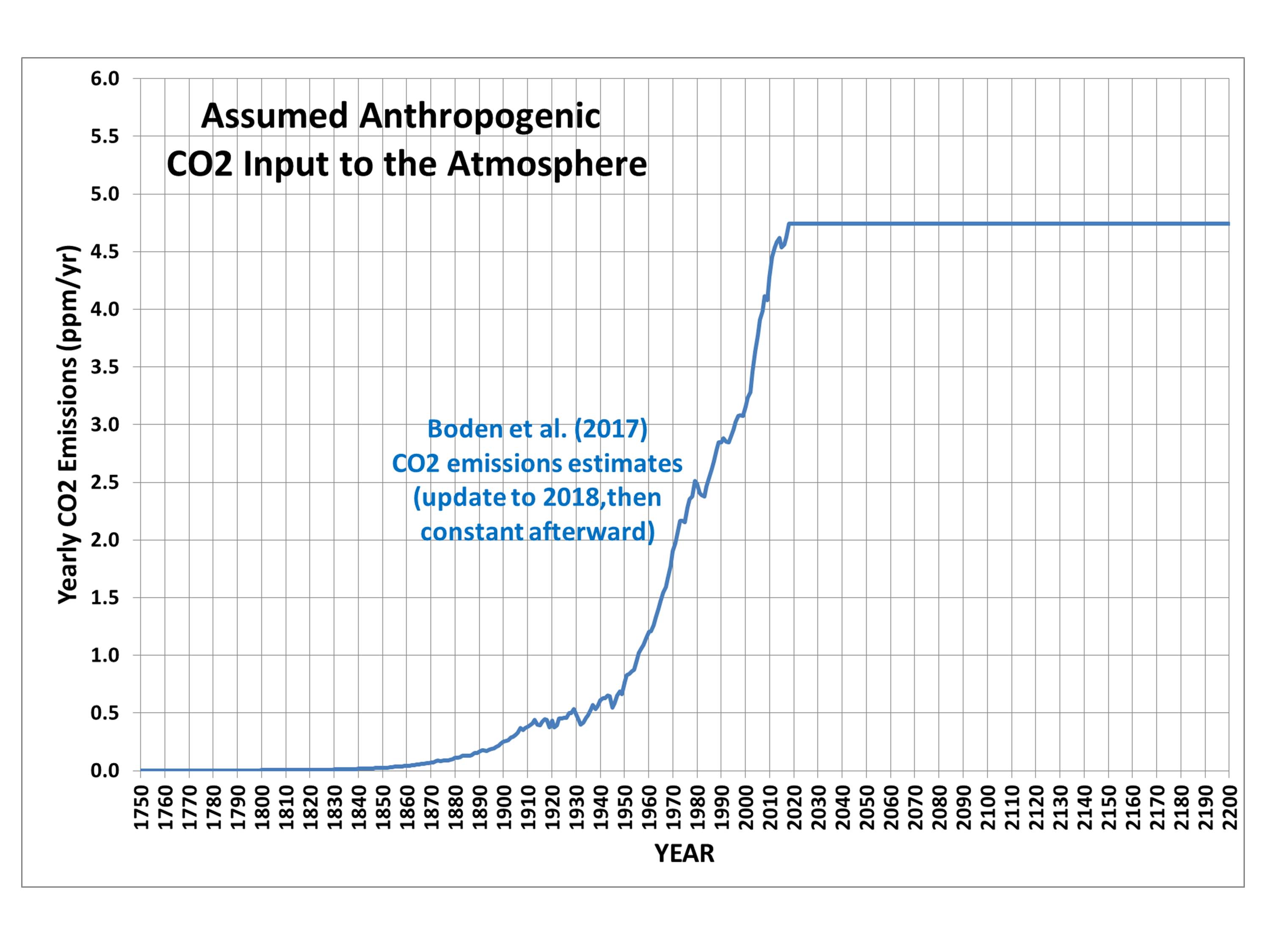
The model uses the Boden et al. (2017) estimates of yearly anthropogenic CO2 production rates since 1750, updated through 2018. The model assumes that the rate at which CO2 is removed from the atmosphere is proportional to the atmospheric excess above some natural “equilibrium level” of CO2 concentration. A spreadsheet with the model is here.

Here’s the assumed yearly CO2 inputs into the model:

Fig. 1. Assumed yearly anthropogenic CO2 input into the model atmosphere.

I also added in the effects of El Nino and La Nina, which I calculate cause a 0.47 ppm yearly change in CO2 per unit Multivariate ENSO Index (MEI) value (May to April average). This helps to capture some of the wiggles in the Mauna Loa CO2 observations.

The resulting fit to the Mauna Loa data required an assumed “natural equilibrium” CO2 concentration of 295 ppm, which is higher than the usually assumed 265 or 270 ppm pre-industrial value:

Fig. 2. Simple model of atmospheric CO2 concentration using Boden et al. (2017) estimates of yearly anthropogenic emissions, an El Nino/La Nina natural source/sink, after fitting of three model free parameters.

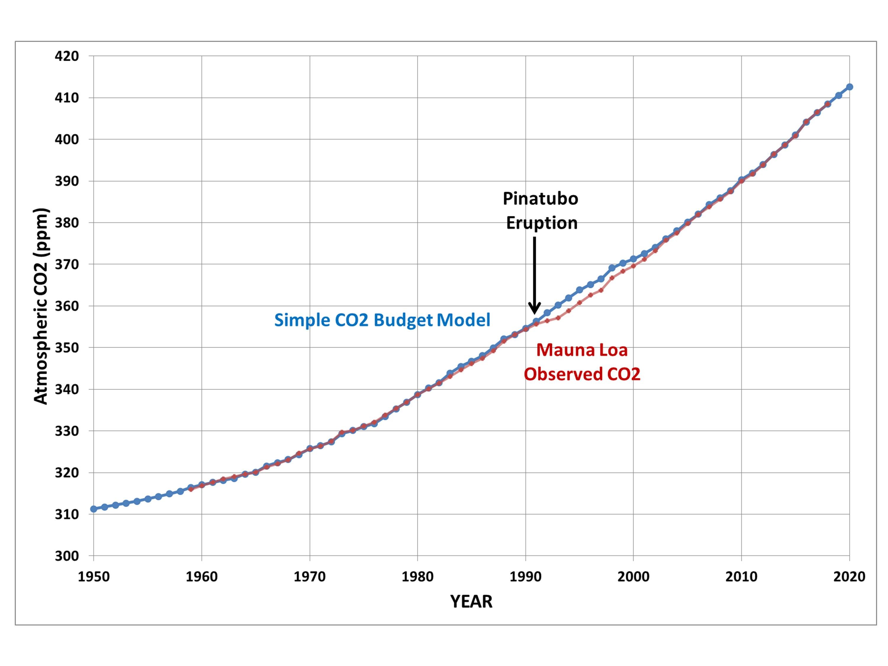
Click on the above plot and notice just how well even the little El Nino- and La Nina-induced changes are captured. I’ll address the role of volcanoes later.

The next figure shows the full model period since 1750, extended out to the year 2200:

Fig. 3. As in Fig. 2, but for the full model period, 1750-2200.

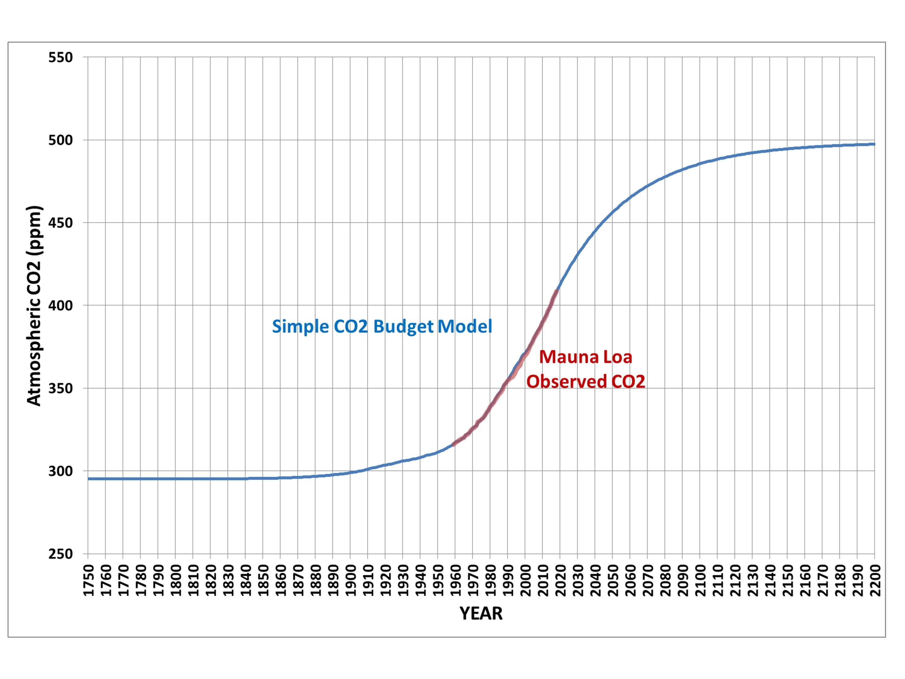
Interestingly, note that despite continued CO2 emissions, the atmospheric concentration stabilizes just short of 500 ppm. This is the direct result of the fact that the Mauna Loa observations support the assumption that the rate at which CO2 is removed from the atmosphere is directly proportional to the amount of “excess” CO2 in the atmosphere above a “natural equilibrium” level. As the CO2 content increases, the rate or removal increases until it matches the rate of anthropogenic input.

We can also examine the removal rate of CO2 as a fraction of the anthropogenic source. We have long known that only about half of what is emitted “shows up” in the atmosphere (which isn’t what’s really going on), and decades ago the IPCC assumed that the biosphere and ocean couldn’t keep removing excess CO2 at such a high rate. But, in fact, the fractional rate of removal has actually been increasing, not decreasing.And the simple model captures this:

Fig. 4. Rate of removal of atmospheric CO2 as a fraction of the anthropogenic source, in the model and observations.

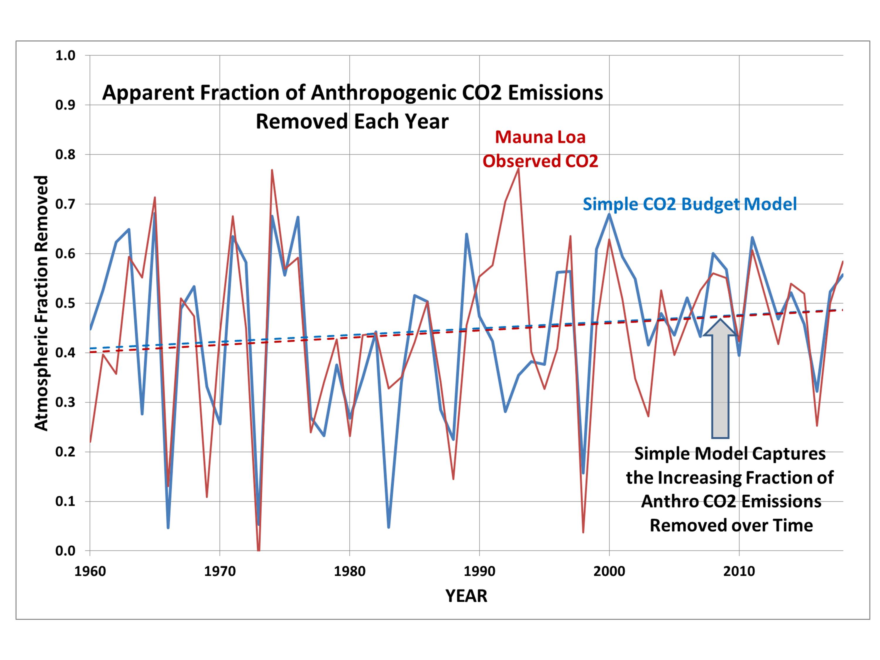
The up-and-down variations in Fig. 4 are due to El Nino and La Nina events (and volcanoes, discussed next).

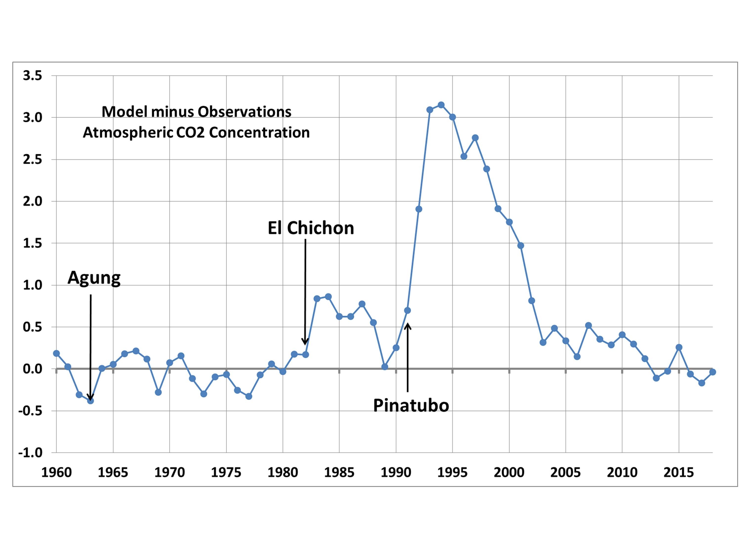
Finally, a plot of the difference between the model and Mauna Loa observations reveals the effects of volcanoes. After a major eruption, the amount of CO2 in the atmosphere is depressed, either because of a decrease in natural surface emissions or an increase in surface uptake of atmospheric CO2:

Fig. 5. Simple model of yearly CO2 concentrations minus Mauna Loa observations (ppm), revealing the effects of volcanoes which are not included in the model.

What is amazing to me is that a model with such simple but physically reasonable assumptions can so accurately reproduce the Mauna Loa record of CO2 concentrations. I’ll admit I am no expert in the global carbon cycle, but the Mauna Loa data seem to support the assumption that for global, yearly averages, the surface removes a net amount of CO2 from the atmosphere that is directly proportional to how high the CO2 concentration goes above 295 ppm. The biological and physical oceanographic reasons for this might be complex, but the net result seems to follow a simple relationship.


651 Responses to “A Simple Model of the Atmospheric CO2 Budget”

Toggle Trackbacks

  1. Entropic man says:

    Nice model.

    Unfortunately you started out with the assumption that CO2emissions would stabilise at present levels.

    This may not be the case. The rate of release accelerated by 1.6% in 2017 and 2.7% in 2018.

    https://www.globalcarbonproject.org/carbonbudget/18/highlights.htm

    The pause in acceleration from 2013 to 2016 may not be representative of the future trend.

    It would be interesting to see the output of a run assuming continued emission increase, perhaps 2%/year.

    • Roy W. Spencer says:

      Oh, I agree completely. I need to take one of the future emission scenarios and see what I get for CO2 concentration, versus what the IPCC gets with their carbon cycle models.

      • Bart says:

        With a dense enough signal base, you can fit any set of signals to any series you want. It isn’t meaningful.

        Occam’s razor argues that the fit requiring minimal data with the fewest assumptions is most likely the right one. And, that fit is simply that the rate of change of atmospheric CO2 is essentially proportional to appropriately baselined temperature anomaly.

        http://tinyurl.com/y6rx2kus

        Our emissions have minimal impact. It’s so obvious. Keep watching that emissions curve, because it isn’t even close to leveling out, and it’s going to keep accelerating going forward. But, atmospheric CO is going to continue doing what it has been doing for the past 60 years – evolving such that the rate of change is essentially proportional to appropriately baselined temperature anomaly.

        • Kristian says:

          I think you’re right, Bart. Because there’s no sign whatsoever in the ToA radiation flux data of any “GHE” strengthening over the last 34 years:
          https://okulaer.files.wordpress.com/2019/01/olr-60-60-erbsceres-c-1.png

          If such hypothetical strengthening had in fact occurred and been the cause of observed warming over this time period (1985-2018), the orange OLR curve would be seen to trend significantly downwards relative to the black TLT curve, gradually and systematically all the way from the start. It clearly and obviously doesn’t. Rather it tracks it tightly.

          This whole bubble will burst sooner or later.

          • Entropic man says:

            To produce the observed warming OLR needs to be 0.7W/M^2 lower than incoming radiation.

            Thatwould translate to a brightness temperature running consistently 0.2C below TLT. You would also see the two graphs running parallel rather than diverging.

            That is well inside the noise level of your data, so that graph is not going to be much help.

          • Kristian says:

            Entropic man says, April 12, 2019 at 8:15 AM:

            To produce the observed warming OLR needs to be 0.7W/M^2 lower than incoming radiation.

            No. It needs to be ~1 W/m^2 lower than what is observed. That orange curve would have to rise by about 1 W/m^2 LESS than what it does, from 1985 to 2018. But it simply rises with the tropospheric temps. Which is what we would observe WITHOUT any kind of discernible strengthening of the “GHE”; i.e. with the null hypothesis.

            You would also see the two graphs running parallel rather than diverging.

            No, then you do not understand how the warming mechanism from an “enhanced GHE” is supposed to work, entropic. Heat loss is supposed to be held back – at equal T_s and T_tropo. That’s the whole point. That’s how warming within the Earth system is supposed to be generated.

            But it doesn’t happen that way. At all. It only happens as the solar heat INPUT increases. As per the data.

            Try again.

          • Nate says:

            As you know, this plot is patched together by Kristian, and it cannot be found anywhere in the literature for this period. You can find one who reconstructs it differently.

            And what happens if you use RSS, instead? Quite a bit of separation will occur.

            The difference in trend is 0.08C/decade x 3.5 decades x 3.85 = 1.1 Watts/m^2.

          • Kristian says:

            Nate, stop trolling. Ever the data denialist. Always quick to butt in with your disruptive nonsense. In your mind, your dogma CANNOT be wrong, so you twist your arguments into pretzels to avoid acknowledging the reality before you, shown in the data. You SEE how tightly the two datasets follow each other, and yet you feel the need to PRETEND that there’s still a systematic divergence because of LINEAR TREND LINES. I mean, how deep does this self-deception of yours run? You’re a religious zealot and nothing else on this issue, Nate.

            Nate says, April 12, 2019 at 11:10 AM:

            As you know, this plot is patched together by Kristian, and it cannot be found anywhere in the literature for this period.

            And as YOU know perfectly well, Nate, there is nothing controversial about this plot: The ONLY thing that I’ve done here is calibrating the baseline of each of the two official OLR datasets used (ERBS Ed3_Rev1 and CERES EBAF Ed4) relative to one another. I’ve simply determined the offset across the five-month 1999-2000 data gap between the two. That’s it. NOTHING ELSE. Everything else is simply the plotting of officially published data.

            And that ONE offset, matching exactly the temperature rise (T_s and T_tropo/TLT) over the gap in question, is thoroughly corroborated by both the HIRS dataset, the ISCCP FD dataset, the AVHRR dataset, Loeb et al., and Allan et al.

            Everyone interested can readily see this for themselves here:
            https://okulaer.wordpress.com/2018/03/24/the-data-sun-not-man-is-what-caused-and-causes-global-warming/

            And here:
            https://okulaer.wordpress.com/2018/06/26/verifying-my-near-global-1985-2017-olr-record/

            All of this you know, Nate. Because we’ve had this exact ‘discussion’ before. And still all you do is try your best to present this plot as somehow just my way of forcing the data to fit with MY agenda. Even though you KNOW your claim is false.

            That’s pretty low. You’re deliberately twisting reality to create your OWN, Nate. To fend off you cognitive dissonance when faced with actual reality.

            It’s sad to see.

            You can find one who reconstructs it differently.

            Not across the relevant section, Nate. The ONE section that I myself addressed; that small 1999-2000 gap between the two datasets. Allan et al.’s offset here agrees perfectly with mine (see second link above). What they do instead is simply change the data of an official dataset (the ERBS Ed3_Rev1), in bulk fashion, simply because they don’t like the look of it – it doesn’t fit with their model. They adjust the data and voil! Lo and behold! It fits. Meanwhile, the people actually responsible for the dataset in question do NOT agree. They have looked into and completely dismiss the (weak, tendentious) reasons given for the change Allan et al. did. They have now even updated the dataset to a new version (Ed4) and specifically kept their internal calibration.

            But you don’t care about that, do you, Nate? Because Allan et al.’s flat OLR model fits with YOUR narrative too. And so no argument to the contrary will ever change your mind.

            And what happens if you use RSS, instead? Quite a bit of separation will occur.

            Sure. When you intentionally adjust TLT data to do just that, disagree with the OLR data, you will of course see separation. But the thing is, it’s pretty straightforward to show that the new RSSv4 TLT dataset is severely flawed, because it’s fundamentally internally inconsistent, while the UAHv6 TLT dataset is perfectly internally consistent and in agreement with the surface series across the main time segment of divergence between the two (1999-2003):
            https://okulaer.wordpress.com/2018/11/11/how-the-ceres-ebaf-ed4-data-disconfirms-agw-in-3-different-ways/

            You’ve got nothing, Nate. Yet you cling to all the straws you can find.

            The difference in trend is 0.08C/decade x 3.5 decades x 3.85 = 1.1 Watts/m^2.

            Hehe, linear trend against the actual data. Only a zealot protecting his doctrine with all means possible would stoop to such childish tactics.

          • Nate says:

            K,

            ‘Nate, stop trolling. Ever the data denialist. Always quick to butt in with your disruptive nonsense.’

            You mean stop interfering in your attempts to present this analysis as a slam-dunk, when you know very well it has flaws, and caveats, and is non-peer-reviewed ?

            You mean don’t bring up issues that require you to put your analysis in proper context, with all required caveats. as you were JUST forced to do?

            Oh, and never mention the cherry picking of UAH over RSS, that completely changes the conclusion?

            OK, cuz, thats trolling..

          • Nate says:

            ‘its pretty straightforward to show that the new RSSv4 TLT dataset is severely flawed’

            If you have to throw out an entire data set, to make your hypothesis work out, that’s generally considered a problem in science.

            If it were that easy to show that RSS were flawed, you should publish that result, but you won’t, because its not that easy.

          • Nate says:

            N: ‘The difference in trend is 0.08C/decade x 3.5 decades x 3.85 = 1.1 Watts/m^2.

            K: “Hehe, linear trend against the actual data. Only a zealot protecting his doctrine with all means possible would stoop to such childish tactics.”

            You are a very weird person, K.

            Feel free to show your analysis with RSS.

            But you will find this difference in trends between UAH and RSS, scsaled by 3.85, because, you know, simple math like this actually works!

            Do you disagree that slope = rise/run?

            And therefore rise = slope x run?

            Or is it the fitting of linear trends that you think is a major sin?

          • Nate says:

            BTW, sho made these ‘trollish’ statements?

            Now, at this stage some might ask and rightfully so why I keep using the UAHv6 TLT dataset only in these comparisons. There are, after all, other tropospheric temperature datasets out there.

            ” we see a fairly obvious gradual and steady increase over time in TLT over OLR, from the relatively low average level of the first 4-5 years to the relatively high average level of the 3-4 years connecting the trough of the 2011/2012 La Nia and the peak of the 2015/2016 El Nio.

            In other words, if the RSSv4 TLT series is correct, the two plots above are both clearly indicating a strengthening ‘greenhouse mechanism’, as radiatively defined, at work in the Earth system.”

            Oh it was Kristian himself…

            Hence, K, desperately needs a way to reject RSS. And right on cue, he finds one.

            He makes a series of hypotheses, really questionable qualitative guesses, about how the TLT record should relate to a surface DWLWR record. A record derived from the CERES satellite record AND weather data AND extensive MODELING.

            And when, after using various arbitrary scaling factors, they don’t behave as he guessed they would, he doesn’t question his hypotheses or scaling factors, or the modeling methods.

            Instead he concludes the TLT data, RSS, must be wrong!

            Wow. Just wow.

          • Kristian says:

            Nate,

            For this one I’ll quote “Bart” from downthread, in also addressing you:

            I don’t know what I can do to help you. It’s like discussing the Moon’s rotation with the other guys. You don’t understand, and you’re not going to understand.

            You’re simply a lost case. Discussing this particular subject with a person as dogmatically blind as you are is the epitome of a Sisyphean undertaking – a complete waste of time and effort.

            You’re not going to understand because you don’t WANT to understand. Rather, you cling to your narrow belief system in everything you do and say, not ready at all to even consider any perspective other than your own. We see this in the way you consistently avoid providing any kind of constructive, objective input on this issue, how instead your only goal in these ‘discussions’ appears to be to shoot down any (ANY!) evidence-based argument that might conflict with your bias.

            That’s the MO of a religious zealot, Nate. That’s YOU.

          • Nate says:

            K, As you know very well, I have raised legitimate science issues with your analysis, some of which made you aware of information. I am a scientist, have published and reviewed papers, and I understand what normal standards in science are.

            IMO, your analysis does not meet the normal standards of science, eg see my comments on your bogus rejection of RSS.

            Cleary you find it easier to attack the messenger, with ad homs than to address the issues.

          • Nate says:

            You accuse me over and over of being a zeolot, mainly because I have heavily criticized your posts.

            Lets face it, both of us have some bias.

            If you look carefully at my posts, you must agree that most of the time I defending science and scientists against so much stupid declarations that people here.

            Nothing religious about that.

          • Nate says:

            ‘your only goal in these discussions appears to be to shoot down any (ANY!) evidence-based argument that might conflict with your bias.’

            I feel exactly the same way about you and Bart.

            The main reasons I push back so hard against you and Bart are:

            1. You guys are both capable of understanding the issues.

            2. You guys keep posting and reposting the same analyses over and over without ever mentioning previous rebuttals.

            3. You guys express WAY WAY WAY to much certainly about your conclusions from these never-peer-reviewed analyses. Way more than professional scientists would. Mainstream science considers uncertainty and error analysis way more than you do.

            4. The ideological motivation underlying your analyses is ever present (see #3). E.g. your implication that RSS scientists, and others, are purposely altering their results.

            5. You both express disdain for mainstream science, and you seem think that its very likely that you, amateurs, have found flaws that many many many professionals, working for many decades have somehow missed. IMO this is ridiculous.

            6. You reject honest criticisms, and (particularly you K) express utter condescension for the peons (such as me) who make them. This attitude ENCOURAGES people to find the flaws in your posts.

          • Dr Roys Emergency Moderation Team says:

            “I am a scientist, have published and reviewed papers, and I understand what normal standards in science are.”

            ☺️

        • Nate says:

          Occam just barfed in his grave!

          Let’s see, which is SIMPLER?

          One idea is we’ve been emitting stuff and it has been accumulating. In the air, ocean and biosphere, at approx the rate of emission.

          While the alternative mechanism is undefined, qualitative, requires unlikely coincidences, and cannot explain where the emitted stuff went, isotopic changes, and much more.

          Hmmm, which would Occam choose?

          • Bart says:

            It hasn’t been accumulating at “approx the rate of emission”. The rate of emission has been about twice as much as the accumulation, and the ratio is increasing.

            It requires no unlikely coincidences, just common, everyday feedback processes.

          • Nate says:

            You didnt read carefully: ‘In the air, ocean and biosphere’

            Coincidences?

            Well, the accumulation rate has tracked the human emission rate, as Roy shows, decade by decade, for 6 decades, and with larger error for 12 decades.

            Carbon has been accumulating in the ocean and biosphere, also tracking the rate of emissions.

            And as noted, the total accumulation matches quantitatively (within uncertainty) to the total emitted.

            The alternative model suggests that these are a streak of coincidences.

            And it suggests that while all the anthro carbon has been gobbled up by nature and hidden somewhere, nature has kindly replaced it, decade by decade, with an identical amount of natural CO2.

            I call this the ‘Body Snatchers’ scenario. IOW it is science fiction, and not even realistic science fiction.

          • Bart says:

            This is pure assertion. We do not measure all the flows. It has been modeled to fit the narrative with what we do measure, but it is not established fact.

            All we can say for certain on that front is that the observed atmospheric rise is roughly 50% of the emissions. So what? It had to be some factor. It happens to be that. All the reservoirs readily accessible to our measurements will show proportionate changes. It’s not a coincidence. It’s tautology.

          • Nate says:

            The whole basis for this nonsense was the meme that ‘Natural flows’ were so much larger than anthro ones, so anthro is just being gobbled up and not accumulating.

            But if ‘All the reservoirs readily accessible to our measurements will show proportionate changes.’ then that means they are finite, and fast equilibrating. And we can see their relative sizes are comparable.

            Thus, they are not so large that anthro emissions are gobbled up and vanishing, as you would like.

            So the raison d’etre for ‘natural only’ model is wrecked.

            Your original claim that

            ‘you can fit any set of signals to any series you want. It isn’t meaningful.’

            is a ridiculous assertion.

            You cannot get the tight tracking of emissions to concentration, that Roy shows, decade by decade, for 6 decades with a simple, physically-motivated mathematical model, and be quantitatively consistent with data, by accident.

            And to boot, your ‘body snatchers’ scenario makes one question your judgement.

          • Bart says:

            The reservoirs that are accessible to us are a fraction of those available. Our measurements of the deep oceans are virtually nonexistent. Of the upper oceans, as well as all the soils and forests and mineral shelfs, spotty at best.

            “You cannot get the tight tracking of emissions to concentration, that Roy shows, decade by decade, for 6 decades with a simple, physically-motivated mathematical model, and be quantitatively consistent with data, by accident.”

            Yes, you can. Easily. The consistency is only in a low order polynomial domain. It is not hard at all to match that.

            What is hard, well nigh impossible, is matching every nook and cranny, as the temperature data matches the rate of change of CO2.

          • Nate says:

            “Yes, you can. Easily. The consistency is only in a low order polynomial domain. It is not hard at all to match that.”

            What is hard, well nigh impossible, is matching every nook and cranny, as the temperature data matches the rate of change of CO2.”

            Like to see you do that.

            It should match as well as it does match.

            Actually Roy DID match every nook and cranny by including an simple dependence of CO2 on ENSO, which have a know causal relationship.

            You seem to have lost all common sense when it comes to this issue.

          • Nate says:

            ‘The reservoirs that are accessible to us are a fraction of those available. Our measurements of the deep oceans are virtually nonexistent. Of the upper oceans, as well as all the soils and forests and mineral shelfs, spotty at best.’

            There are measurements, but you ignore them, because you dont need observations to confirm your beliefs.

            If you look at the measurements you would see that the carbon flows to the deep ocean don’t work with your models.

            The reservoirs that are accessible to us, are the fast equilibrating ones. Precisely the ones that matter.

            These are the ones that make the large natural flows that we see every year, and which are the basis for the whole meme that the natural flows are SO MUCH BIGGER, that causes a few deniers to think human emissions are too small to matter.

          • Bart says:

            Actually Roy DID match every nook and cranny by including an simple dependence of CO2 on ENSO, which have a know causal relationship.

            Its more than just ENSO. The correlation between temperature and rate of change of CO2 holds in the long term as well. It matches both the variation and the trend ever since reliable and accurate measurements became available at MLO.

            Dr. Spencers match comes at the expense of ignoring that striking, long term correlation, and in essence arbitrarily filters it out in favor of anthropogenic inputs at low frequencies.

            This is not only arbitrary, but it treats natural and anthropogenic inputs on a different level, with natural inputs being removed more rapidly than anthropogenic ones. That is not kosher. Continuity must be preserved.

            The reservoirs that are accessible to us, are the fast equilibrating ones. Precisely the ones that matter.

            No. This is a slowly evolving increase in atmospheric CO2. Those are precisely the ones that dont matter.

            You seem to have lost all common sense when it comes to this issue.

            I havent. If I strike you as one of those thoughtless, knee-jerk deniers such as those who have regularly thread-bombed these pages with simple-minded naysaying, (and who apparently, and blessedly, have been banned as they do not appear to be making an appearance here), then you should by all means simply ignore me.

            If, however, I appear to have anything at all on the ball to you, perhaps you should consider my inputs seriously, let go of your biases for a while, and try to look at the evidence objectively.

          • Nate says:

            ‘If, however, I appear to have anything at all on the ball to you, perhaps you should consider my inputs seriously, let go of your biases for a while, and try to look at the evidence objectively.’

            You are on the ball mathematically, but you have shown a repeated tendency to ignore data and simple logic that doesnt fit your narrative, eg isotopes, ocean measurements, ice cores.

            IOW, your rationality and ability to look at evidence objectively is what I seriously question.

            Lets just take your principle claims:

            You assert, without evidence, that all or most of the emitted carbon has been removed by nature.

            You further argue that nature has replaced this removed carbon, by NEARLY the same amount, decade by decade for 6 decades!

            You don’t see this as improbable, as any sensible person would.

            You assert that this highly improbable scenario agrees with Occam’s razor, when entirely the opposite is true!

            You want to argue that the close quantitative matching between emissions and accumulation is no biggie, just mother nature playing a huge practical joke on us.

            C’mon, that is just insane.

          • Bart says:

            you have shown a repeated tendency to ignore data and simple logic that doesnt fit your narrative, eg isotopes, ocean measurements, ice cores.

            These are merely circumstantial. They do not rise to the level of the smoking gun seen in the plot of the rate of change of CO2 and temperature anomaly.

            You assert, without evidence, that all or most of the emitted carbon has been removed by nature.

            The evidence is that CO2 is being driven by the above temperature relationship, and there is very little room to shoehorn in an additional anthropogenic dependence.

          • Bart says:

            You further argue that nature has replaced this removed carbon, by NEARLY the same amount, decade by decade for 6 decades!

            Roughly half the amount. That’s not “nearly the same amount”.

            Its just some number. It has to be some number. It happens to be this one. Thats not hugely improbable.

          • Bart says:

            You want to argue that the close quantitative matching between emissions and accumulation is no biggie, just mother nature playing a huge practical joke on us.

            There is no close quantitative matching. There is just the 50%, and it is assumed the rest went somewhere else. I can do what with anything.

            My gas tank is half full. The rest must have spilled out. Never mind that I drove 200 miles yesterday. I have a quantitative match between the amount in my tank, and the amount spilled out, so you cannot doubt that it spilled. That is the level of your argument.

            The things you think are improbable are not improbable at all. The things you think are likely are actually highly improbable, when you actually understand how natural systems generally work.

          • Bart says:

            Let’s move any further discussion to the bottom. It’s annoying having to search for and scroll up and down on this one.

          • Nate says:

            N “Actually Roy DID match every nook and cranny by including an simple dependence of CO2 on ENSO, which have a know causal relationship.”

            B: “Its more than just ENSO. The correlation between temperature and rate of change of CO2 holds in the long term as well. It matches both the variation and the trend ever since reliable and accurate measurements became available at MLO.”

            No, actually it doesnt match without extra fiddling with arbitrary filters that reduce fast variation. That is NOT kosher.

            Roy’s matches well to the decade by decade acceleration, and most of the faster variation, except the 90s, as noted. You are simply denying this.

            “Dr. Spencers match comes at the expense of ignoring that striking, long term correlation, and in essence arbitrarily filters it out in favor of anthropogenic inputs at low frequencies.”

            He is using a minimal model connecting 2 things that have a known CAUSAL relationship. He does consider ENSO temperature as well. No need for anything else, other than large volcanic eruptions.

            “This is not only arbitrary, but it treats natural and anthropogenic inputs on a different level, with natural inputs being removed more rapidly than anthropogenic ones. That is not kosher. Continuity must be preserved.”

            How so? Not arbitrary at all. No additional ‘natural inputs’ are needed to obtain an excellent fit, except for volcanic activity (which he could have tried to model and include)

          • Bart says:

            I have already addressed these points. They have no merit.

    • Stephen P Anderson says:

      This model looks like a nice model. The guy spent a lot of time on it. But, it is not of this world. He took a preconceived notion that all the CO2 increase is anthropogenic and constructed a model to fit that narrative. He had to assume a residence time of at least 52 years and also very low natural CO2 emission. One thing I’ve learned is that the planet consumes CO2. It doesn’t hang around long. The belief that all of this 150ppm rise in CO2 is anthropogenic requires low natural emission and a very long residence time. That is not this world.

      • Stephen P Anderson says:

        If anthropogenic emission gets really high-25 times more than it is right now, you’d expect CO2 to level out at about 800ppm as long as natural emission does not rise. I think the estimates are that anthropogenic emission can only get to about 3 times what it is now or about 15ppm. So, natural emission is the driver. Temperature has caused natural emission to increase. What caused the temperature rise? Don’t know but it wasn’t CO2.

  2. Alick says:

    Wouldn’t CO2 molecules and H20 molecules have a tendency to separate in the atmosphere with H20 above the CO2 due to their difference in mass?

    • Roy W. Spencer says:

      No, because gas molecules are so small. In the presence of any atmospheric turbulence, gases of different molecular weights are uniformly distributed with height. Even small particles of rock (dust) can stay suspended for weeks, and they are very much larger than gas molecules.

      • Alick says:

        I can’t argue with how you see it. I am just saying gravity is always exerting force on these molecules whether we see the effect or not. and I would argue that we do see the result of this effect when we look at clouds.

        If you could set a CO2 molecule and an H20 molecule inside an empty cylinder, say half-way up. Step 1: apply an equal upward force to both for the same amount of time, (keep in mind gravity is also working on both molecules) then the H20 molecule will wind up higher than the C02 molecule. 2) If you then take away those upward forces at the same time and only allow gravity to work for a short time on both molecules, they will both fall at the same rate with the vertical difference between them achieved from step 1 remaining the same. Repeat Step 1.

        You’d be hard pressed to tell me that Steps 1 and 2 are not constantly being applied to CO2 and H20 molecules (really every molecule) in the atmosphere. The presence of other molecules to bump into, or magnetic fields, only masks what I know must be going on at a foundational level.

        • bohous says:

          The equilibrium density distribution of molecules in the absence of any turbulence would be governed by exponential function exp(-mgh/kT) where m is the mass of one molecule. For two types of molecules the ratio of densities Rho1/Rho2 would be controlled by exp(-(m1-m2)gh/kT). Nevertheless, the ekvilibrium is not achieved fast enough to be able to fight the turbulence in the atmosphere, at least at low altitudes.

          • Alick says:

            What turbulence? Collisions with other molecules, molecules to the same gravitational force?

            Aside, you know I’ve always wondered that if you were placed in a little pocket of air at 14.7 psi at the center of the Earth, would you feel gravity pulling you apart in all directions, or crushing you from all sides?

      • Nate says:

        Alick,

        Once molecules mix, they don’t easily unmix. Thermal agitation and entropy won’t let them.

        Put sugar in your coffee, without stirring. Its heavier, so sugary coffee settles on the bottom.

        Now stir it. Check a day or two later. Equally sugary on top and bottom.

        It hasnt unmixed, and won’t for as long as you can watch.

        • Alick says:

          Nate,

          Liquids have bonds that make them liquids, so I don’t view it the same. Gases to my understanding are molecules that have broken the bondage of being a solid or liquid, usually through the input of energy. With enough “thermal agitation” to your sugary cup of coffee and I’d wager I could separate the water molecules from it leaving the sugar on the bottom.

        • Nate says:

          Yeah, sometimes interactons betwwen molecules becomes stronger than thermal agitation, like with oil and water. They are unhappy mixed.

          But, sugar and water happily mix. As do CO2 and Nitrogen and Oxygen. Good thing, if not, we’d have only co2 down here at the srface and all nitrogen up high.

          • Alick says:

            Nate,

            That would suck to have all the CO2 down here.

            Once, my brother and I threw a softball size piece of dry ice in a 55 gallon drum (cylinder on end) with a few inches of water in the bottom. It made a fog about 3/4 the way up the barrel. What do you think a couple of curious kids that didn’t know any better tried to do next? lol Damn right, we stuck our heads in the fog and tried to breath.

            I like your examples. I’m hearing that you think gases in the atmosphere behave like sugar in water rather than like oil in water.

            I think they behave more like oil in water. Why does the oil rise to the surface of the water? You have to remember that the atmosphere is constantly having energy put into it from the sun. For the sake of consistency we need to continuously shake that container of oil and water.

            Hopefully you can understand that just because we are shaking the oil and water mixture and everything looks equally mixed, the proclivity for the oil to rise to the top of water doesn’t stop being there, it is just masked by the shaking. Same goes for Co2 and H2o molecules in the atmosphere, IMHO.

            All those clouds we see in the sky are formed from water vapor (single H2o molecules) that have risen up through CO2, I’m just explaining a mechanism for how it happens.

          • Nate says:

            Fun story..

            ‘I think they behave more like oil in water. Why does the oil rise to the surface of the water?’

            Oil molecules are attracted to each other. In a shaken up mixture they only have to move a short distance to find other oil molecules to stick to. After awhile good sized droplets form.

            A big droplet of oil weighs less than water so it rises. If it were heavier it would fall (settle).

            As Roy noted, small objects settle much more slowly than big objects.

            So a human’s terminal velocity thru air is larger than a cat’s, which is larger than a bug’s. A molecule has a ridiculously tiny terminal velocity (settling velocity).

            https://upload.wikimedia.org/wikipedia/commons/thumb/3/3f/Settling_velocity_quartz.png/1280px-Settling_velocity_quartz.png

            While at the same time, molecules have very high random thermal velocities, like 300 m/s.

            So they are constantly being mixed up.

          • Alick says:

            Nate,

            This post will probably wind up out of order.

            The density matters. What is density but a ratio of mass/space.

            I think you missed the point of the oil and water being constantly shaken to simulate the energy of the sun constantly bombarding Earth. Shake faster to simulate for more sunlight or slower for less, it really doesn’t matter, because the point is no matter how hard you shake, you can’t shake out of existence that the oil wants to be on top of the water.

            To simplify, two things can be true at the same time while shaking that oil and water mixture; 1) the oil and water can “look” thoroughly mixed and 2) the oil is always working to be on top of the water. Just as H2O wants to be on top of CO2 in the atmosphere even though it isn’t what we measure; but we do see it everyday in the formation of clouds that once began as water vapor from the surface.

            You know those rooms for children full of balls, that’s essentially what the atmosphere is. A cylinder full of balls, the walls off the “container” being gravity.

          • Alick says:

            “Thermal velocity” isn’t a vector, it’s a scalar.

          • Nate says:

            “2) the oil is always working to be on top of the water. Just as H2O wants to be on top of CO2”

            Not really. The opposite. When enough oil molecules stick together, the droplet rises.

            When enough water molecules stick together, in a cloud, they fall.

            The difference is water went thru a phase change and became liquid, which happens at the dew point, which happens at some height in the atmosphere.

            Clouds are not showing water on top of air or CO2, just showing water condensing at some height where its cold enough.

          • Alick says:

            “Not really. The opposite. When enough oil molecules stick together, the droplet rises.”

            Not if you keep vigorously shaking the jar.

  3. Nate says:

    Nice work!

    Wondering about the 295.

    It seems Bodens data is pretty flat before 1850.

    Is he perhaps not including the effects of deforestation for the centuries leading up to 1850?

    • Nate says:

      Might it also have to do with having fast and medium and slow removal rates?

      • Roy W. Spencer says:

        yes, I suppose the model cannot address any slow CO2 removal processes which are not significantly impacting the 60 years of Mauna Loa data.

        • Svante says:

          This model includes slow removals:
          – Deep ocean overturning.
          – CaCO3 neutralization.
          – Silicate weathering.

          https://tinyurl.com/y54wl3hv

          The long term effect on temperature depends on total emission, not rate.

          • Stan says:

            Svante, What model assumptions account for the delay between t=0 introduction (to the atmosphere?) of the slug of CO2, and its t=33y peak concentration in the atmosphere?
            (Thanks, Roy, I know this is a bit off-topic for this thread.)

          • Svante says:

            Hi Stan.

            That would be inertia in the climate system, we have about thirty years of warming in the pipe line.

            This is not a full climate model, in reality there are long term feed backs that will keep adding for hundreds of years.
            For example, two degrees will wipe out most of the Greenland ice sheet, but it will take thousands of years.

    • Entropic man says:

      Nate

      Based on British Antarctic Survey data, for most of the last milennium CO2 content was stable at about 280ppm.

      It then started to rise about 1800 and has accelerated since.

      https://www.bas.ac.uk/wp-content/uploads/2015/04/002.jpg

      This agrees quite well with Dr Spencer’s suggestion that without human perturbation the “natural” level of CO2 for the present interglacial is around 280ppm.

    • Entropic man says:

      “Removal” is perhaps the wrong word.

      CO2 is not removed from the atmosphere in any permanent sense. It transfers to the ocean or the biosphere. The three reservoirs exchange CO2, trying to reach equilibrium.

      At present human CO2 output mostly enters the atmosphere first, then about half of it transfers to the other reservoirs, so the total amount in all three reservoirs increases.

      If geoengineering started to reduce the atmospheric CO2 content, then all that “removed” CO2 would return to the atmosphere.

      • Dave Burton says:

        Entropic man wrote, “If geoengineering started to reduce the atmospheric CO2 content, then all that removed CO2 would return to the atmosphere.”

        No, only a small portion of it would return to the atmosphere, because the additional carbon would be distributed across the various carbon reservoirs, and only a small portion of the carbon is in the atmosphere. E.g., there’s about 50x as much CO2 in the oceans as in the atmosphere.

    • Dave Burton says:

      The 295 might reflect the fact that mankind has added quite a bit of long-sequestered carbon to the Earth’s active carbon reservoirs: air, oceans, biosphere, etc.

      The amount of carbon we’ve added to the atmosphere is large compared to the amount that was already there, but small compared all the active carbon reservoirs, combined.

      If there were no exchange between those reservoirs, we’d be approaching a doubling of atmospheric CO2 level, by now, from the CO2 mankind has added. But there’s a lot of ongoing exchange between the reservoirs. Over half of the CO2 which mankind has added to the atmosphere has already been removed from the atmosphere by those transfers to the biosphere, oceans, etc.

      “Equilibrium” atmospheric CO2 level should be expected to be a bit higher, now, than it was before we burned all that coal and oil.

      Of coarse, other things affect the equilibrium, as well. Warmer ocean water temperatures shift CO2 from the ocean reservoir to the air. Milder & more equable climates regimes shift CO2 from the air into the biosphere, as vegetation expands. Biological processes which sequester CO2 in calcium carbonate remove CO2 from oceans. Et cetera, et cetera, etc.

      But it would be surprising if adding all that CO2 had not raised the equilibrium atmospheric CO2 level a bit, and 295 ppmv is a plausible level.

  4. matthew dalby says:

    Presumably if emissions keep rising then the total amount of CO2 will stabalise but at a level slightly above 500ppm. The model throws into question if we will ever see CO2 levels reach double the pre-industrial level, so even if the IPCC estimates of equilibrium climate sensitivity are correct (I seem to remember a central figure of about 2 degrees for a doubling of CO2) then it is highly unlikely that we would see more than aprox. 1.5 degrees of anthropogenic warming. If all of the post 1970’s warming is anthropogenic then the maximum amount of future warming would be a maximum of 1 degree, plus almost 1 degree of warming since the 1850’s therefore it is likely that we could meet the goals of the Paris agreement (limiting warming to 2 degrees above pre-industrial levels) without doing anything.

    • Roy W. Spencer says:

      I didn’t mean to imply we wouldn’t reach 500 ppm, since it’s unrealistic to assume CO2 emissions won’t keep rising, probably for decades to come. I just wanted to see how high CO2 would go under a simple assumption: a constant rate of emissions. I didn’t expect the level would stabilize…although it’s obvious why when I think about it.

      • Entropic man says:

        It is obvious if you assume, as your model does, that the proportion of CO2 in the ocean and biosphere will increase relative to the atmosphere as the total CO2 in the three reservoirs increases.

        This may not be the case.

        The equilibrium between atmosphere and ocean depends on Henry’s Law, which says that the two come to equilibrium at equal partial pressures. A doubling of atmospheric CO2 would beexpected to produce a doubling of dissolved CO2. This isa linear relationship, not the non-linear relationship you assume. There is also the problem that decreasing pH also decreases the amount of dissolved CO2 the ocean can hold.

        The equilibrium between atmosphere and biosphere depends on how increased CO2 affects photosynthesis. Once again, this is a linear relationship only if CO2 is the limiting factor. Unfortunately plants encouraged to grow more by increased CO2 rapidly run into other limits; light, nutrients, temperature and water. I doubt that a higher CO2 world biomass will store as high a proportion of total CO2 as it does now.

        Overall the proportion of CO2 leaving the atmosphere may decrease, rather than increase.

        • Bart says:

          It is not so simple. The oceans are immense, and equilibration takes centuries. In the near term, only the upper strata can equilibrate with the atmosphere. The rest takes centuries. And, the oceans have enormous buffering capacity.

          • Dave Burton says:

            I agree with Bart.

            Entropic man wrote, “…if you assume, as your model does, that the proportion of CO2 in the ocean and biosphere will increase relative to the atmosphere as the total CO2 in the three reservoirs increases.”

            Roy’s model does not assume that.

            Perhaps you meant to write “level” instead of “proportion”?

            As the atmospheric CO2 level rises so does the rate at which it is removed by dissolution into the oceans (a <a href="negative/stabilizing feedback). You’re not doubting that fact, are you?
             

            E.m. continued, “A doubling of atmospheric CO2 would beexpected to produce a doubling of dissolved CO2. This isa linear relationship, not the non-linear relationship you assume.”

            Assuming unchanging temperatures and no other CO2 sources or sinks, then as the CO2 levels in the air-ocean system approach equilibrium, the levels in the air would be falling and the levels in the oceans would be rising. But because the oceans contain about 50 as much CO2 as the atmosphere, the atmospheric CO2 level would fall much more rapidly than oceanic CO2 level would rise.
             

            E.m. continued, “There is also the problem that decreasing pH also decreases the amount of dissolved CO2 the ocean can hold.”

            I’m no chemist, but it is my understanding that the opposite is true: chemical buffering reduces pH changes, and makes the amount of CO2 the oceans can hold essentially infinite.

            However, if water temperatures rise, that would shift the equilibrium. Equilibrium would be reached at a slightly higher atmospheric CO2 level and lower dissolved CO2 level than would be the case with unchanging water temperatures.
             

            E.m. continued, “The equilibrium between atmosphere and biosphere depends on how increased CO2 affects photosynthesis. Once again, this is a linear relationship only if CO2 is the limiting factor. Unfortunately plants encouraged to grow more by increased CO2 rapidly run into other limits; light, nutrients, temperature and water.”

            That’s wrong. It is easy to create contrived circumstances where other things are limiting factors, but, in the real world, overall, on planet Earth, CO2 shortage will always be the main limiting factor, for plant growth.

            CO2 levels would have to rise far above plausible levels for that to cease to be the case. Optimum for most plants is about 1500 ppmv or above.

            That’s believed to have been the approximate average CO2 level during the lush Cretaceous; during the Jurassic levels are thought to have been even higher.

            Not coincidentally, that’s also a typical target for daytime levels in commercial greenhouses (achieved by the use of CO2 generators).

            W/r/t/ water, higher CO2 levels reduce water requirements and increase drought-resistance of plants.

            W/r/t temperature, warmth generally accelerates growth. Warmer climates have longer growing seasons and are, on average, lusher than colder climates. The fact that things like trees and corals tend to grow faster when it is warmer, and slower when it is colder, is what enables us to count “growth rings” to determine their ages.
             

            E.m. continued, “I doubt that a higher CO2 world biomass will store as high a proportion of total CO2 as it does now.”

            Actually, it will almost certainly be even higher. It takes a while to grow trees, so a sharp increase in atmospheric CO2 level leads eventually to a corresponding increase in biomass, but the biomass growth lags the CO2 level increase.

            Rising CO2 levels are already “greening” the Earth, but it’s just getting started.
             

            E.m. continued, “Overall the proportion of CO2 leaving the atmosphere may decrease, rather than increase.”

            Not possible. As long as CO2 levels increase, so will the rates at which negative feedbacks remove CO2 from the atmosphere.

  5. Fredrik says:

    Does it matter in this model (and in the real world) whether the emissions are coming from fossil fuels or alternative (bio) fuels?

    • Roy W. Spencer says:

      I suppose if it was coming from biofuels and new biomass was continuously being grown to replace the burned biofuels, then the rate of uptake by vegetation would be even higher, and it would lower the CO2 levels.

      • Fredrik says:

        OK, I understand, but if the rate of influx from burning biofuels is higher than the rate of uptake by vegetation, the CO2 in the atmosphere would increase anyway right?

        If the CO2 increases due to burning fossil fuels, wouldnt the rate of uptake from vegetation increase with a similar amount then, i.e., even if one does not intentionally plant new plants the vegetation would increase by itself (by more growth in forests, lands, and waters)? So it would not matter for the CO2 level in the atmosphere whether the influx is coming from fossil fuels or not.

        But maybe this is out of topic for this article? Sorry in this case!

        • yes, you are correct. Burning is fast, growing is slow. Only in the long term can the growing absorb what had been burned. At least that’s my initial impression.

          • stan says:

            “Burning is fast” [e.g. << 1 y]",growing is slow" [e.g. 1~10 y] — compared to these, further equilibrations like surface temperature or ice accumulation or deep oceans, may be much much slower.

          • Svante says:

            The CO2 thermostat will fix the current spike within a million years.

        • Entropic man says:

          Fredrik

          On topic, methinks. Ultimately this topic is about the carbon cycle.

        • Nate says:

          Apparently planting trees may cause MORE warming. Trees have low albedo compared to grassland.

          • Dave Burton says:

            Trees have many effects. They change the albedo of the land. They convert radiant energy into chemical energy (hydrocarbons). They remove CO2 from the atmosphere. They transpire water, which increases heat transport to the mid-troposphere (where the water vapor condenses in clouds), and which might affect cloud cover. They produce particulates (especially right here, right now, where I live).

            The largest effect of trees on temperatures might be at northern tree lines. Boreal forests are dominated by evergreens. Since they remain green even when there is snow on the ground, boreal forests have much lower albedo (i.e., they are darker) than unforested ground, in snowy conditions, hence they absorb more sunlight. If a warmer climate causes tree lines to advance toward higher latitudes, this should be a positive feedback mechanism in those regions:

            warmer temperature → increased forestation → lower albedo → warmer temperature

            (This feedback is mentioned in the 7th paragraph of p.4 of Grantham’s Briefing paper No 12, June 2015, Biosphere feedbacks and climate change.)

            Of course, were’re mainly talking about Siberia and northern Canada, where, by any sane standard, it’s too darn cold. So a few more trees, and a little bit of resultant warming, there, is a Good Thing.

      • gbaikie says:

        And biofuels emit more CO2 per energy produced. So if replacing coal one will emit more CO2 [and more pollution] for same amount of energy. And worst if replace natural gas with biofuels.

  6. Brian Harrison says:

    Learn why “greenhouse” gases (water vapor, carbon dioxide) can only COOL the surfaces of Earth and Venus. This ( https://youtu.be/bT1iFhGKOI8 ) is the ONLY video with correct science about temperatures and heat and what causes natural climate change. Please watch it in full (15 mins) as it will blow your mind. It outlines a whole new paradigm in what is common thinking about the role of Solar energy and how that energy even keeps the core of the Moon far hotter than its surface. The author’s world-first discovery of a “heat creep” process turns conventional thinking on its head. Please pass this on to all your friends and colleagues: nobody will ever prove it wrong, but it certainly proves climatologists wrong with their fictitious, fiddled physics.

    Doug Cotton, why do you have to pretend to be someone else? Do you really think you are fooling people? -Roy

  7. Bindidon says:

    It certainly won’t take much time until this very interesting contribution is reposted at WUWT.

    I’m sure Ferdinand Engelbeen will read the stuff there.
    I’m curious what he’s going to say about it!

    • Bart says:

      He will regurgitate his narrative, based upon a grab bag of facts and wishful thinking.

      • Bindidon says:

        You never were able to accurately contradict him.

        • Bart says:

          I did. His model requires treating natural and anthropogenic inputs differently. Ferdinand is no dynamicist. He does not understand requirements on continuity for physical realizability. He just throws darts at a board.

  8. Very nice work. Get’s the essential dynamics right.

    The most likely explanation for the higher equilibrium value of 295 ppm is that this value is temperature dependent. And caused by the one degree celcius warming during the last 100 years.

    And fits well with the changes of about 6 degrees celcius and the corresponding change of CO2 of 100 ppm during the ice ages = 100/6 ppm pr. degree = app. the increase from 280 to 295.

    So to make the model complete you need to include the temp vs. CO2 relationship.

    Yes, I agree. I just don’t know how to quantify that. Some temperature effect has already been taken out indirectly from using the MEI data. -Roy

    • Entropic man says:

      “So to make the model complete you need to include the temp vs. CO2 relationship.”

      The difference between a glacial period with ice to 50N latitude and the current interglacial is 80ppm CO2 (200ppm then, 280ppm befor 1850)

      Most of this is stored in tundra peat and permafrost during the cold part of the cycle, relaesed into the atmosphere during the long thaw, and absorbed again as the ice returns. The transition usually takes about 10,000 years, which is rather long term by modern standards.

      • Dave Burton says:

        A lot of it is probably in the oceans. Colder water results is a bit more CO2 dissolved in the oceans, with a bit less remaining in the atmosphere; warmer water has the opposite effect.

  9. DMA says:

    So what controls the “natural equilibrium level”? If the controller changes then the level will change. Salby shows that the controller is temperature. Harde and Salby show that most of the increase is natural not human caused. Munshi shows that the atmospheric concentration is not responsive to changes in rate of emissions so human emissions must be much smaller than natural and appear to be lost in the noise of the varying natural sources. There is no data that would lead us to believe that sinks are reaching saturation as the C14 generated by the bomb tests decayed exponentially in a little over 10 years. I have not seen a reasonable refutation of these of Dr. Berry’s work and Humlum’s work shows temperature leading CO2 at even short time frames. I don’t think the rate of human emissions plays more than a minor role in the atmospheric content at any time.

    How can you say “the atmospheric concentration is not responsive to changes in rate of emissions”, when I just showed near-perfect agreement between the two in a simple model? Also, just because CO2 is rapidly cycled between the surface and atmosphere (as evidence by 14C data, and even the IPCC says about 30% of atmospheric CO2 is removed — and replaced — every year), this is NOT what controls how fast EXCESS CO2 in the atmosphere is removed. The model I presented suggests it takes about 70 years for 2/3 of the extra CO2 to be removed (if I turn off all emissions after 2018) – Roy

    • Entropic man says:

      Under past natural conditions the glacial/interglaial transitions changed CO2 by 80ppm in 10,000 years (0.008ppm/year). Temperature led CO2.

      Current conditions are not comparable. Fossil fuels are releasing 4ppm/year gross, 2ppm net, and CO2 is leading temperature.

      • DMA says:

        There is good reason to question the CO2 change rates in ice cores. Other sources give vastly different results. There is solid analysis to conclude that the currant CO2 rise is mostly natural. If it were all due to anthropogenic emissions the changes in emissions would be reflected in the atmospheric growth rate and they are not. Look over (https://edberry.com/blog/climate-physics/agw-hypothesis/contradictions-to-ipccs-climate-change-theory/ ) or watch (https://www.youtube.com/watch?time_continue=3937&v=rohF6K2avtY ) for an introduction to this analysis.

        • Bindidon says:

          DMA

          Wow! One paper by Ed Berry is enough for you to doubt about the work like

          https://cdiac.ess-dive.lbl.gov/trends/co2/lawdome.html

          This is simply ridiculous. What the heck do such observations and their accurate processing have to do with your recurrent “IPCC has it all wrong” ?

        • Entropic man says:

          DMA

          This paper makes the old error.

          CO2 leaving the atmosphere does not conveniently disappear.

          The atmosphere, ocean and biosphere form three coupled reservioirs in equilibrium, with constant exchange between them. You cannot consider one in isolation and get sensible conclusions.

          • DMA says:

            I don’t think the work of Salby or Berry says that the CO2 from the atmosphere is destroyed or somehow permanently sequestered when it is absorbed out of the atmosphere. Their work is aimed at analyzing the characteristics and components of that flow. Their results, if valid, draw the conclusions I referred to above. I can not see why their model is invalidated by lumping all extra-atmospheric effects on CO2 as outside the box. If you want to model a reservoir level you do not need to know what goes on outside the reservoir. All that is necessary is inflow and outflow.
            Your concept of the three reservoir being in equilibrium requires a very long time reference I believe.
            Thank you for your response.

          • Curious George says:

            That’s why the simple empirical relationship Dr. Spencer found is important. It allow us to bypass all the gory details.

    • DMA says:

      Roy
      Thank you for responding. I have studied all of Muraay Salby’s videos and Hadre 2017 and, although I am not qualified to adequately parse their work, I can’t find fault with it. The analysis of Munshi at (https://tambonthongchai.com/2018/12/19/co2responsiveness/ ) are the work I rely on for the statement about response to emissions. I don’t think Kohler’s response to Harde is convincing and the journals response to Harde’s reply is horrible (https://hhgpc0.wixsite.com/harde-2017-censored ). Why is Salby’s analysis of the CO2 flow in the atmosphere in error? Why is it inappropriate to to consider a one box model like these scientists do? Why doesn’t the Bern model of flow not work on known data?
      I really would like to get to the truth but have not seen this work refuted well and think that should be a focus because if they are right the rest is so much arm waving.

    • Bart says:

      “…when I just showed near-perfect agreement between the two in a simple model?”

      It’s not “near perfect”. It’s just vaguely in the same direction. With enough curve fitting parameters, you can always get that. Differentiate it to put the signals into the rate domain, and you will see there is hardly any consilience at all.

      “…The model I presented suggests it takes about 70 years for 2/3 of the extra CO2 to be removed”

      You cannot just assume arbitrary dynamics, and accept whatever gives you a vague fit. It must take the same amount of time for natural inputs to be removed as anthropogenic. If it took this long for natural inputs to be removed they, being far greater proportionately, would have driven levels much higher than they are long ago.

    • swampgator says:

      Because correlation does not equal causation?

      • Nate says:

        Indeed, please explain that to Bart.

        Four things are correlated, temperature, emissions, atm concentrations, ocean concentrations.

        What are the causal relationships between these?

        Bart’s hypothesis is temperature CAUSES atm and ocean concentrations, but he can only arm-wave about the mechanism.

        He cannot explain what CAUSES the temperature to rise, again arm waving only.

        He cannot explain the correlation to emissions, it is just happenstance, however, an extremely improbable one.

        IN sharp contrast, standard science explains that emissions CAUSE atm concentrations to rise which CAUSES ocean concentrations to rise and CAUSES temperatures to rise.

        The CAUSAL mechanisms are clear, physically based, and quantitative, and most importantly, have corroborating evidence.

        No correlations are left as improbable happenstance.

        • Bart says:

          Conjecture is not explanation. There are vast volumes of writing that spin worlds and scenarios that form cohesive narratives. The book industry puts out thousands every year. You can find them under “Fiction” in your local bookstore.

          The facts are, concentration is not rising consistently with emissions, and temperatures are not rising consistently with the models.

          • Svante says:

            In other words, emissions are rising, concentrations are rising, and temperatures are rising.

        • Nate says:

          ‘Conjecture is not explanation.’

          Your model for what is happening is almost ENTIRELY conjecture.

          ‘There are vast volumes of writing that spin worlds and scenarios that form cohesive narratives.’

          The vast volumes are filled with data, and analyses, and physics based models, built over many decades that are pieces of the puzzle.

          What you call ‘spin’ and ‘scenarios’, and of course trying to find a cohesive narrative that fits the facts, is ordinary science in action.

          Perhaps in ~ 1900, with Arrhenius, and maybe 1938 with Callendar, you could call their ideas conjecture.

          But too much evidence has been gathered since then, so much has been learned about the carbon cycle, ocean and atmospheric dynamics.

          Calling that hard-won understanding of the Earth CONJECTURE is just ridiculous.

  10. Jeff says:

    “CO2 is removed from the atmosphere is proportional to the atmospheric excess above some natural equilibrium level of CO2 concentration”

    Yes, this has always been my belief, but I don’t think this is so central to other CO2 modelling.

    In general the higher the concentration of chemical, the faster the reactions that use the chemical will tend to happen.

  11. Gerard says:

    We nneed to revisit Henry’s Law. This determines the partion between gasses in the liquid and gaseous phase. As concentration in the atmosphere increases the system compensates to absorb more in the liquid phase.

  12. Entropic man says:

    The Drax power station in England burns 4 million tons of wood pellets each year.

    A Sitka spruce plantation yields 150 tons/ acre after 40 years.

    4 million tons is equivalent 40 square miles of Sitka spruce plantation burned each year.

    To make Drax carbon neutral you would need 1600 square miles of spruce plantation, cutting and replanting 40 square miles each year.

    • Bindidon says:

      Which power class does your Drax belong to? 500 MW?
      At which load does it work? 70%?

      Then to be honest I would prefer a mix of offshore wind units and gas!

      • Entropic man says:

        Bindidon

        The biomass section of Drax has a capaxity of 2.6GW. It produces about 4% of total UK electricity consumption, 15% of our renewable output.

        • Bindidon says:

          Thanks for the clarification.

          Biomass represents in Germany also a lot of RE, actually a bit more than onshore wind.

          But over the long term, it is considered to be a blind-alley: electricity production is only about 15% (!) of the total consumption.

          • Entropic man says:

            Bindidon

            In the short term, burning biomass tends to return CO2 previously absorbed by biomass to the atmosphere. In the long term, 40 years+, the sort of management regime I described would be viable and carbon neutral. It would be analogous to coppiceing birch woodland to produce a steady supply of firewood.

            In the long term we’ll need all the different renewables. Even ignoring climate change issues, fossil fuels are a finite resource which will run out.

            Anyone claiming that our civilization cannot function without oil is setting a time limit. When the oil runs out, civilization stops!

    • Adam Gallon says:

      Drax is one huge subsidy farming device.

      • Bindidon says:

        Adam Gallon

        “Drax is one huge subsidy farming device.”

        Aha.

        … and what do you think about the ‘subsidiy level’ of nuclear-based electricity production during the last 50 years?

        Apart from the fact that lots of nuke plants were ‘decommissioned’, but still none of them was DISMANTLED with success.

        To give you a nice little hint: the French 4G breeder Superphénix was shutdown in 1997, and at that time its dismantling costs still were estimated at incredible 300 MFRF i.e. about 50 M$.

        The operation started in 2007, with a new estimate of 1 G$ (yes: factor 20), and operation’s end was predicted for 2027.

        But in over ten years, they still did not manage to finish the very first major step, namely to properly get rid of 5500 tons of highly contaminated liquid sodium used in the primary cooling system.

        Imagine the nuclear industry would have to pay for Fukushima’s consequences…

    • Nate says:

      “1600 square miles of spruce ”

      Interesting!

      Wonder, what would 1600 sq miles of PV solar produce?

      Use 10% efficiency (some empty spaces)

      Peak power: 1600 mi^2 *(1609 m/mi)^2 * 100 W/m^2 = 4 x 10^11 W

      Average power ~ 1 x 10^11 W

      US peak power is 10^12 W average power 4×10^11 W

  13. Hans Erren says:

    Hi Dr Spencer,

    Based on the Vostok icecore data I would suggest a temperature dependent equilibrium of 280 + 16*T ppm (with T temperature relatime to preindustrial)

    That gives 296 ppm equilibrium for the year 2013.

    Try SRES A1T for future emissions which is similar to the Nordhaus optimum emission scenario.

    See my modeling using a similar approach as yours and using Lewis&Curry sensitivities in the url under my name.

    • Bindidon says:

      Sounds good to the layman…

    • Entropic man says:

      Hans Erran

      Where is the increase in temperature coming from?

      UAH V6.0 is showing warming of 0.13C/decade. Since 1979 that is an increase of 0.5C, at a rate of +1C every 76 years.

      The consensus explaination is CO2 forcing. I have yet to find an alternative explaination for this temperature rise which stands up when you calculate the energy involved.

  14. Steve Fitzpatrick says:

    Hello Roy,
    I did essentially the same thing many years ago in a guest post at WUWT in its early days. I fitted my model using an assumed pre-industrial CO2 level of ~280-285 PPM, historical CO2 emissions estimates, and historical variation in average sea surface temperature (which captures the effects of ENSO and volcanoes on short-term CO2 uptake). Yes, with just a couple of parameters you can get a remarkably good fit to the historical CO2 record. But that said, the logical basis of this kind of simple model may not be physically realistic, and so the ability of the model to project future concentrations of CO2, especially in the long term, is dubious at best. Other models of CO2 uptake (eg the Bern model) seem to me little better… just curve fits with very questionable physical basis. The hard questions, like how the rate of CO2 sequestration by plants (land and aquatic) will change over many decades, and how much thermohaline overturning and turbulent down-mixing of surface waters each contribute to ocean dissolution of CO2, now and in the future, remain unanswered.

    By the way, my long-ago post at WUWT was a direct responce to you suggesting most increase in atmospheric CO2 was a result of outgassing due to a slight warming of the ocean surface… which struck me as nonsensical.

  15. Petit_Barde says:

    Another simple model may be based on the assumptions that :
    – CO2 concentration evolution is mainly due to temperatures evolution,
    – according to Henry’s law, and since oceans are 71% of the Earth’s surface, CO2 concentration increases when T increases and vice versa,
    – the guess that when temperatures increase, the biomass increases and thus also the CO2 concentration,
    – CO2 emissions by volcanoes may (and do) act on CO2 concentrations, but the guess is that this interaction is rapidly absorbed (some months to some years) and thus should not impact much (in the long run) the relation between CO2 and T,
    – there also seems to be a discrepancy between T and instantaneous CO2 concentration rates because of hemispheres asymetry (mainly with respect to seasons, sun irradiance with respect to seasons, biomass, oceans/soils). In order to tackle this, we should take a 12 months mean of CO2 concentrations.

    The simplest function describing how the CO2 concentration rate evolves with respect to temperatures T is a linear function of the temperature T. This gives us the following dissipation equation :

    d[CO2]/dt = a*T + b

    where a and b are constants,
    T is the global mean lower troposphere temperature anomaly,
    [CO2] is the 12 months mean CO2 concentration.

    This simplistic model can be tested here :

    http://www.woodfortrees.org/plot/esrl-co2/from:1979/mean:12/derivative/plot/uah5/from:1979/scale:0.22/offset:0.14

    Used constants :
    a = 0.22
    b = 0.14

    • Entropic man says:

      Petit_Barde

      You get the same result with

      dT/dt = a*[CO2] + b

      The problem is that you are discussing correalation, rather than causation. Without a clearly understood mechanism you cant say which is the cause and which is the effect.

      • Petit_Barde says:

        Entropic man,

        the simple model I propose is based on sound assumptions (e.g. Henry’s law, biomass increase with temperatures, which all together may explain some of the causality T -> CO2) and on what a dissipation equation looks like (the time derivative on [CO2] is not the result of a random guess).

        Conversely, (and I would say, as expected) you obtain nothing with :

        dT/dt = a*[CO2] + b.

        You can test it here :

        http://www.woodfortrees.org/plot/esrl-co2/from:1979/scale:0.001/offset:-0.35/plot/uah6/from:1979/mean:12/derivative

        • Entropic man says:

          Petit-Barde

          Somehow you managed to detrend the UAH data.

          This is what the graph should look like.

          http://www.woodfortrees.org/plot/esrl-co2/from:1979/every/scale:0.007/offset:-2.5/plot/uah6/from:1979/every/plot/uah5/from:1979/every/trend

          • Bart says:

            You made the error. You did not differentiate the temperature data, in accordance with your model.

          • Entropic man says:

            Bart

            I use the consensus forcing formula.

            ∆T=5.35ln(C/Co)climate sensitivity/ forcing response

            ∆T is the change in temperature.

            C is the final CO2 concentration.

            Co is the initial CO2 concentration.

            Climate sensitivity is the multiplying effect of feedbacks

            Forcing response is the forcing wattage change required to warm the climate by 1C.

            Thus the increased CO2 since 1880 would be expected to produce

            ∆T = 5.35ln(411/280)3/3.7 = 1.66C

            Because of the effect of the ocean heat sink there is a lag between a change in CO2 and the resulting change in temperature.

            If you calculate the temperature curve due to increasing CO2 and plot it on the same axes as observed temperatures, the curve derived from CO2 matches the observed curve with a 25 year lag.

          • Bart says:

            The model you said would fit, to which Petit_Barde objected, was

            dT/dt = a*[CO2] + b

            That is not the model that fits. The model that fits is

            d[CO2]/dt = a*T + b

            It fits every nook and cranny, not just some vague low order polynomial. The latter easily produces spurious correlation. The former does not, and is therefore to be preferred.

          • Bart says:

            I mean, do you really not see?

            “If you calculate the temperature curve due to increasing CO2 and plot it on the same axes as observed temperatures, the curve derived from CO2 matches the observed curve with a 25 year lag.”

            Pitiful. You’ve basically got an affine match via affine transformation. This is a triviality. Every affine function is affinely similar to every other affine function.

            Petit-Barde’s plot matches everywhere:

            http://www.woodfortrees.org/plot/esrl-co2/from:1979/mean:12/derivative/plot/uah5/from:1979/scale:0.22/offset:0.14

          • Entropic man says:

            Why is CO2 leading temperature in your graph?

            Surely if temperature were causing CO2 it wouldbe the other way round?

          • Bart says:

            That’s not CO2. That’s the derivative, a.k.a. the rate of change, of CO2.

      • Nate says:

        Petit_Barde,

        ‘Henrys law’ predicts a rise in CO2 concentration that is a small percentage, ~ 3% for 1 degree C of warming.

        https://en.wikipedia.org/wiki/Henry%27s_law

        Thus a 45 % rise in CO2, 280 to 410 ppm, cannot be explained by a temperature rise of 1 C.

  16. Mark B says:

    “The resulting fit to the Mauna Loa data required an assumed natural equilibrium CO2 concentration of 295 ppm, which is higher than the usually assumed 265 or 270 ppm pre-industrial value”

    Observations from the Law Dome ice core suggest atmospheric concentrations were around 280 ppm at the time your model run starts. This suggests it might be unwise to over interpret outside the calibration region.

    • Nate says:

      I agree. The past emissions are pretty uncertain.

      I found that if I let the initial (1958) level, the rate, and the equilibrium level be free parameters, I get the best fit of

      C_1958 316.4
      rate: 0.0216
      C_0: 289.1

  17. Regarding the statement of 265 or 270 PPM being an assumed equilibrium level of CO2: I have heard mostly 280 PPM for pre-industrial CO2.

    Meanwhile, Willis Eschenbach modeled 283 PPM as an equilibrium level, and time constant of 59 years (half-life of 41 years) assuming that a pulse (injection) of CO2 into the atmosphere gets absorbed by the oceans, etc. in a manner described by exponential decay.

    He also said this does not disprove the Bern model. The way I see it, atmospheric concentration of CO2 will closely follow both the Bern model and the exponential decay of surplus CO2 model while emissions are increasing in a manner close to an exponential curve. However, part of the longer term and permanent parts of the “tail” of projections using the Bern model assume an amount of climate sensitivity to increased CO2 that I consider as greater than it probably actually is.

    This is in:
    https://wattsupwiththat.com/2015/04/19/the-secret-life-of-half-life/

  18. climanrecon says:

    Neat, am I right in thinking that by removal of CO2 you mean the NET effect of molecules leaving the atmosphere and “natural” molecules entering it? If so then the model makes sense, molecules will leave at a rate directly proportional to the concentration, and “natural” molecules will enter at a rate that doesn’t care about the concentration.

    • climanrecon says:

      I can now answer my own question in the affirmative, having looked at the spreadsheet. In effect an assumption is made that “natural” CO2 molecules enter the atmosphere at a constant rate (neglecting El Nino), independent of the atmospheric CO2 concentration, the simplest model one could adopt, and one consistent with a perturbation approach, a “green” nirvana of a steady world having to deal with a small amount of “pollution”.

  19. Trevor says:

    This is counter intuitive. I would have expected following a volcanic eruption that the measured co2 concentration would be higher (not lower) than the model because volcanoes add carbon dioxide to the atmosphere.

    • Entropic man says:

      On average annual volcanic CO2 emissions areabout 1% of human emissions.

      The cooling effect of aerosols is greater than the warming effect of the CO2, so the net effect is cooling.

      By van T’Hoff’s a cooler ocean surface can dissolve more CO2. The net effect of a volcano is therefore a slight reduction in CO2.

      Mind you, we are talking about a Pinatubo. A Tambora or a Yellowstone would be a net CO2 increaser!

  20. Interesting theory.

    However, you seem to assume that the carbon sinks are inifinite, and that is a huge assumption.

    The big question is whether the sinks will saturate at some point. We can model the ocean saturation rate from our knowledge of the ocean surface water and deep water mixing rate, but to model the saturation in the biosphere is an even more challenging exercise.

    /Jan

    • Curious George says:

      Is there an infinite supply of carbon?

      • Good point.

        The carbon resources in fossil fuel are of course not infinite, but they will last for a long time. No peak production are in sight for oil and gas, and the worlds coal reserves are enormous.

        We may get a problem if the fossile reserves last much longer than the eventual saturation of carbon sinks.

        /Jan

  21. Greg Goodman says:

    Dr Spencer, this pre-industrial value you find is very interesting. It is exactly what I found in 2014 using a different method, which I posted here:

    https://climategrog.wordpress.com/co2-log-rise/

    This method leads to a pre-industrial estimation of 295 ppmv. Somewhat higher than the usual estimation of about 280 ppmv.

    I’m trying to track down where I detailed the method.

    • Greg Goodman says:

      Basically I took the log of accumulated emissions according to CDIAC and scaled it fit MLO observations. I took the log of CO2 and found three distinct exponential growth periods described the record quite well.

      The intercept of the earliest growth period intercepted y axis at a value corresponding to 295 ppmv.

      No ENSO, no volcanoes, no account of the excess above base value. A unique scaling factor is applied, being inferred from MLO period which covers the latter two growth periods: essentially 1900-1960 and 1960 onwards.

      The MLO does rise a little faster than the model near the end ( a result of the choice of fitting period ). This probably explains why my extrapolated 2050 is slightly lower at 462ppmv.

  22. Ray Tomes says:

    The temperature of the oceans also affect CO2 levels because child water can hold more gasses. If you use the previous years temperature (out change in it) you can explain CO2 changes more accurately still. In my own study, change in temperature precedes change in CO2 by 6 months.

    • Greg Goodman says:

      Hi Ray, haven’t seen your name in a while.

      Yes d/dt(CO2) does correlate quite well with SST on the interannual scale. This is the out-gassing effect. What you need to take note of is the underlying rate increase in CO2 on which the wiggles are superimposed. That was about 1ppm/year in 1970 and is about 2ppm/year now.

      https://climategrog.wordpress.com/ddt_co2_sst/

      It looks even better if you go to higher differentials:
      https://climategrog.files.wordpress.com/2013/05/d2dt2_co2_ddt_sst1.png

      • Bart says:

        That “underlying rate” fits, too:

        http://tinyurl.com/y6rx2kus

        There is no need for anthropogenic additions to explain any of it, though I expect it accounts for a few ppm more or less. There is simply a bias toward assuming that we are driving it, because most of us live in cities and imagine the entire, vast globe is like that. But, in fact, human habitation spans only about 10% of the total land mass, and 3% of the entire globe.

        • Greg Goodman says:

          Oh dear, my posts are getting dumped.

          • Bart says:

            The site filter is quirky, and is triggered off of phrases or letter combos that were characteristic of site trolls. One thing you can do is save your posts, then if one gets rejected, post it piecemeal until you find the part that offends.

          • Nate says:

            ‘No, I am saying these are imperfect measurements, that come with their own frequency content.

            Now its ‘there is nothing wrong with my model, its the measurements that are imperfect..’

            Look, there is nothing wrong with the measurements.

            What we see clearly is that the response of CO2 to temperature is STRONGER at high frequencies, eg ENSO frequencies.

            That is what is observed.

        • Svante says:

          And the 1st and 2nd derivative were centered around zero before the industrial revolution.

          Why? Because 280 ppm was stable.

          • Greg says:

            … and temperature was not constant, it was rising. Oh dear.

          • Bart says:

            That’s redundant. But, there is scant evidence for it. All the eggs are in the ice core analysis basket. That basket has holes in it.

          • Bart says:

            Nonlinear systems also can experience shifts in operating regimes. We could speculate all day.

            The bottom line is, the best, most modern, most direct, most accurate measurements show that at least since the beginning of the MLO record, the rate of change of atmospheric CO2 is proportional to appropriately baselined temperature anomaly. As that is the era in which the lion’s share of the rise has been observed, that’s really all we need to conclude that anthropogenic inputs have had at most minor impact.

          • Nate says:

            Well actually, if you don’t cheat, as Bart knows very well, the relationship does not hold at all.

            https://tinyurl.com/y2ebovbk

          • Bart says:

            That dog doesn’t hunt.

          • Nate says:

            What youve plotted is self-deception, and straight up fraud. You should know better.

          • Bart says:

            I understand you are frustrated, but the F-word is beneath you. You should be careful how you hurl that one around. It could get you into serious trouble someday.

          • Nate says:

            I use it appropriately.

            You use arbitrary high pass filtering, to reduce the high frequency variability of CO2 while leaving the low frequency untouched.

            This of course, allows you to (artificially) obtain a frequency-independent scale factor.

            Which is supposed to be your main finding!

            Yes it is fraud, and would never pass real peer review.

          • Nate says:

            Sorry not ‘high pass’. ‘low pass’

            while applying NO filtering to temperature data.

          • Bart says:

            The temperature data are already filtered, as is indicated by the match in resolution. Your resolutions are inconsistent.

            You can’t just wish the relationship away, Nate. It is a match, using a minimum of adjustable parameters. It exists. You are howling at the Moon.

          • Nate says:

            “The temperature data are already filtered, as is indicated by the match in resolution.”

            Nope, absolutely false.

            What you call ‘resolution’ is just noise in the derivative not present in temp.

            Its very simple, obtain a 1 y average for each data set, as I do, then plot.

            With your 24 mo smoothing of co2 data, enso variance is significantly supressed.

          • Nate says:

            Why do you need a 24 mo filter for co2 and 1 mo. for Temp?

            Suppose we make it 12/1 for co2/T

            Heres what you get:

            https://tinyurl.com/y6qse9ty

            The relationship disappears.

            Can you explain this?

            Clearly the ENSO variation is less filtered at 12/1, and then requires a different scale factor, and then it is no longer correct for scaling the trend.

            So the ‘effect’ requires 24/1. But what is the objective reason for this setting?

          • Bart says:

            Sure, I can explain it: you changed the scale factor and offset. Change them back to what they were, and the match reappears. It’s more noisy with 12 month filtering, but it’s there.

            These surface temperature data are very noisy, and require more filtering than the much better behaved satellite data to provide a good match. Basically, the better the data, the better the match. That’s what you would expect for a valid relationship.

            You’re barking up the wrong tree here, Nate, if your object is to gain understanding. If your object is simply to pollute the discourse to drown out inconvenient facts, I can’t stop you.

            But, whether the relationship is what you think it should be or not, it is nevertheless there, and it is way too good a fit to be mere happenstance.

          • Bart says:

            You know what, upon looking at the plot again, I realize I got that wrong. It’s not that the surface data are noisier, it’s that they have less resolution. You have to filter the CO2 data down more to match the resolution of the temperature data. Probably due to the fact that there are relatively so many fewer sample locations than for the satellite data. Less information = lower resolution.

          • Nate says:

            Bart,

            I believe you know what the effect filters have. They reduce noise AND signals in a highly frequency-dependent way.

            They are multiplying a signal by a frequency-dependent scale factor!

            You can clearly see here the effect of a 12 mo vs a 24 mo filter on the CO2 data (bottom two curves) with equal scaling factors.

            https://tinyurl.com/yykg78ys

            It should be absolutely clear that to match the top temperature curve, the two bottom curves require DIFFERENT scaling factors.

            This filtering, being strongly frequency-dependent, does not affect the long term trend. Therefore, in one case, 24 mo, you may get a scale factor that roughly is what is needed to get trends to match.

            While for the 12 mo case, the scale factor no longer works for the trends to match.

            Accurately testing whether two data sets have a frequency-independent scale factor is rendered impossible when you have applied a strongly frequency-dependent scale factor to one of these.

            Do you NOT see that?

          • Bart says:

            All it says is that the surface data are low resolution, and more filtering is needed to get the CO2 data to have the same resolution.

            Using the best, highest resolution data we have from the satellites, we get a better fit with less smoothing. That is as it should be.

            If you say the CO2 data does not match the surface data set, you are also saying the surface data set does not match the satellite data. Tell us something we don’t know. They are different measurements, but the satellite data are more representative, because they sample a lot more of the Earth.

            You are clutching at straws. The rate of change of CO2 is proportional to appropriately baselined temperature anomaly. Deal with it.

          • Nate says:

            The resolution of the surface data is definitely not 24 months, and you know that.

            Its time resolution is not determined by how it looks to you. Its time resolution is its averaging time, which is 1 month, same as the satellite data.

          • Nate says:

            The satellite data is measuring the troposphere, which is not the source of the added co2.

            And it is well known that the troposphere has a much stronger response to ENSO, compared to the surface.

          • Nate says:

            With unbiased filtering, this what we get for UAH.

            https://tinyurl.com/yyobf7nx

            No match.

            You will undoubtedly say:resolution.

            If you look at 1998 peaks, you see that thay have the same shape and full width half max-ie the same temporal resolution.

            You need to understand what effect filtering is having, before reaching a conclusion about frequency independence.

          • Bart says:

            “Its time resolution is not determined by how it looks to you.”

            How it looks to you is, indeed, a measure of the resolution. Resolution is determined by the frequency content of the signal. Higher resolution signals have higher frequency content. When you look at a signal and see it is smoother than another, that is an indication that it has lower resolution.

            You are clutching at straws. The rate of change of CO2 is proportional to appropriately baselined temperature anomaly. Deal with it.

          • Nate says:

            ‘When you look at a signal and see it is smoother than another, that is an indication that it has lower resolution.’

            OMG, extremely amateurish.

            When you look at a signal and see it is smoother than another that indicates it has less noise.

            Taking a derivative of data is well known to produce a noisy signal. And sure enough it is noisier.

            It makes absolutely no sense to arbitrarily assume a 24 mo resolution for data that was sampled/averaged monthly!

            The simplest and most logical thing to do with this data is simply look at 12 mo running means for EACH data set.

            With this unbiased approach no one can complain that you are screwing up the frequency-dependence of the relationship between the two data sets.

            But if your goal is achieve a desired result, by any means necessary, then you are committing scientific malpractice!

          • Nate says:

            Here is a good example, the 2015 El Nino, in Temp and CO2 derivative.

            https://tinyurl.com/y4uvw9u9

            The top Temp has 4 mo. smoothing.

            The bottom Temp has 24 mo. smoothing.

            The CO2 derivative has 24 mo smoothing. It has more noise.

            Does the CO2 data match better to the 4 or 24 mo smoothed temperature?

            I think you can clearly see that the 4 mo. smoothed temperature has better time resolution than the other two curves.

            The 24 mo smoothed CO2 data, though more noisy, has a similar time resolution to the 24 mo. smoothed temp data.

          • Bart says:

            Ha ha. No.

          • Bart says:

            You really do not know what you are talking about, Nate. You are just trying to find excuses to deny the obvious. You need a shrink, not me.

          • Nate says:

            “You really do not know what you are talking about, Nate.

            Sounds a lot like JD, when he tells physicists to ‘go learn some physics’.

            That does not apply here. Analysis of time series, noise, and signal processing is a big part of what I do in my day job, so actually I do know what I’m talking about.

            ‘ You are just trying to find excuses to deny the obvious’

            I think that is exactly what you are doing.

            It is obvious to me that 1 mo temp data has much higher resolution than 24 mo smoothed CO2 data.

            It is OBVIOUS in the bloody plot!

            https://tinyurl.com/y4uvw9u9

            It is obvious to me that applying arbitrary filters, is a good way to screw up a frequency-dependent effect!

            If you want to overturn a major scientific paradigm, then you can’t do it with a HALF-ASSED attempt at analysis, like this.

          • Bart says:

            “Analysis of time series, noise, and signal processing is a big part of what I do in my day job…”

            Then, you have a lot of learning to do. First, you need to recognize that these signals have different resolutions ab initio. Resolution depends on more than just sample period. Resolution has to do with the frequency content of the signals. Sampling limits the resolution to the Nyquist frequency, but the sampled signals themselves have their own intrinsic resolution.

            You are trying to put me into a double bind in which I have to match both the surface data and the satellite data without any difference in processing. But, this is an impossible task, because these signals themselves have differing resolution, and do not match each other.

            It’s all just an excuse to avoid dealing with what is plainly evident: The rate of change of CO2 is proportional to appropriately baselined temperature anomaly. Now, deal with it, and don’t bother me anymore with these flimsy non-issues. I’m not interested in helping you out any further.

          • Nate says:

            ‘It’s all just an excuse to avoid dealing with what is plainly evident: The rate of change of CO2 is proportional to appropriately baselined temperature anomaly.’

            You seem to think repeating an assertion like this makes it a fact, no matter what problems it may have.

            But we are finding (and agreeing) that it all depends how you massage the data and which data set you use.

            The obvious data set to use is surface data, because:

            1. CO2 is stored in surface reservoirs. These are the ones you claim are responding to temperature.

            2. Surface temp data goes back further, and allows you to check the dependence for 60 y.

            If the ‘effect’ is not seen in surface data, then it is not there.

            ‘these signals have different resolutions ab initio. Resolution depends on more than just sample period. Resolution has to do with the frequency content of the signals.’

            The frequency content can include noise.

            I understand that MAY be the case, but then you need to find some way to determine the ab initio resolution.

            Do some Fourier analysis.

            It is not kosher to just make it a fitting parameter, and adjusting it to achieve a desired result.

            Resolution will be reflected in the response perturbations, like El Nino.

            You can see it here, 3rd page, comparison ENSO to Global Temp.

            http://www.columbia.edu/~mhs119/Temperature/T_moreFigs/Nino34+Tglb_2014-2019.png

            Definitely it is resolving sub 1 year perturbations with high resolution.

          • Nate says:

            ‘First, you need to recognize that these signals have different resolutions ab initio.’

            Actually, I don’t understand what you mean here.

            The sensors measuring Earths temperature have very high temporal resolution, thermometers: minutes, satellites: hours.

            So it can’t be the MEASUREMENT of temperature that you mean.

            Do you mean that the Earth’s temperature has slow response times, to perturbations?

            If that’s what you mean, I agree.

            But your hypothesis is that CO2 derivative is responding to Earth’s temperature.

            Now you are saying it is responding FASTER than temperature itself. How can that be? That makes no sense.

            If it is responding faster than temperature, then it is responding to something else, not temperature.

          • Bart says:

            I’m only going to respond this one more time, because you have gone off the deep end, and this conversation has become merely annoying.

            Resolution is both spatial and temporal, and they are coupled. E.g., averaging a traveling wave function over a wavelength is equivalent to averaging over a period.

            Stop looking for excuses to disbelieve your eyes. The rate of change of CO2 is proportional to appropriately baselined temperature anomaly. Deal with it.

          • Nate says:

            is your model, as youve stated it many times:

            “The rate of change of atmospheric CO2 is proportional to appropriately baselined temperature anomaly.”

            Now you are saying at high frequecies, the relationship is somehow modified, to enhance the response to temperature that we actually measure.

            The temperature is naturally filtered, but co2 responds to the unfiltered version of temperature?

            How convenient!

            Whatever your speculative model is, you are admitting that low and high frequencies need a different scale factor.

          • Bart says:

            No, I am saying these are imperfect measurements, that come with their own frequency content. The better the measurements, the better the fit with less preprocessing, as we see with the satellite data vs. the surface data.

          • Nate says:

            “No, I am saying these are imperfect measurements, that come with their own frequency content.”

            Now its the ‘there is nothing wrong with my model, its the measurements that are imperfect..’

            Look, there is nothing wrong with the measurements.

            What we see clearly is that the response of CO2 to temperature is STRONGER at high frequencies, eg ENSO frequencies.

            That is what is we see.

          • Bart says:

            No, it isn’t. There is a very good match between the satellite data and the d[CO2]/dt derivative as I have shown repeatedly, and they have the same resolution, because they are both averages over 1 year equivalent.

          • Nate says:

            “No, it isnt. There is a very good match between the satellite data and the d[CO2]/dt derivative ”

            This is like JD saying a black body is also a mirror.

            Simply a denial of reality.

          • Nate says:

            ‘because they are both averages over 1 year equivalent.’

            Even this is a denial of facts.

            You averaged co2 for 2 years!

            Consider a sine wave of amplitude 1, period 3 y, which matches the peak of ENSO spectrum.

            The 2 y running average will reduce the amplitude of the sine wave to 0.4.

            A 60% reduction.

          • Bart says:

            “You averaged co2 for 2 years!”

            For comparison with the lower resolution surface data, not for the satellite data. The satellite data is higher resolution and higher quality, and that is where the fit is the best. That’s what you expect for a valid model.

            The model cannot fit both the surface and the satellite data, because they do not fit each other. If we can only choose one, the satellite data is the one we want to fit best. And, we do.

          • Bart says:

            “Simply a denial of reality.”

            Utter nonsense. The fit with the satellite data is very, very good.

          • Nate says:

            FYI Bart,

            I found this data for the South Pole atm CO2. It looks just like Mauna Loa but it and its derivative are much less noisy.

            Take a look, how does its resolution look to you?

            https://cdiac.ess-dive.lbl.gov/ftp/trends/co2/sposio.co2

          • Bart says:

            It’s pretty low resolution.

            We don’t have great data. The CO2 data is at most from a few points. The temperature anomaly data are global bulk measurements, with the satellite data far more comprehensive.

            It’s a wonder there’s a match at all. That there is a very good one tells me that the SNR is quite high for the impact of temperature anomaly on the rate of change of CO2.

            You don’t get this kind of agreement through happenstance. There is definitely a strong relationship here. And, this is how dissipative systems striving for balance typically work. There’s not some static pot that just sits there and collects what we put in. That notion was created by climate guys who are not clued into how dynamic systems typically evolve. Just a bunch of overspecialized dudes creating models of spherical cows.

        • Svante says:

          Greg says:
          “and temperature was not constant, it was rising.”

          No, temperatures were in decline, good thing we turned it around, pity we overdid it.

          https://tinyurl.com/yc35hg66

  23. Stephen P Anderson says:

    Explain to me how the absorber differentiates between a natural CO2 molecule and a anthropogenic molecule?

  24. Stephen P Anderson says:

    The first fatal flaw in the model is that it implies a residence time of 52 years. So if preindustrial equilibrium level is 280ppm then 280/52 is 5.3ppm of natural emission. We know this is/was impossible.

    • Bart says:

      You are correct, Stephen. Under this presumption, natural inputs account for about 300 ppm, and our puny inputs, estimated to be on the order of 30x less or a greater factor, accounts for 100. Emissions are in a ratio of perhaps 30:1, but impact is presumably on the order of 3:1.

      To get that kind of disparity, one would have to have a grossly nonlinear feedback response with polynomial order of about 10. With that kind of feedback power, CO2 concentration would be extremely sensitive to tiny upsets, like even a small volcanic eruption. Nowhere in the record do we see such extreme sensitivity.

      The whole thing is absurd. Perhaps decades from now, people will mock this scare as akin to phlogiston and fears of sailing off the end of the world. It is that stupid.

      • Stephen P Anderson says:

        Yeah Bart, I’m not sure what planet this model belongs to but it is not this planet.

      • Nate says:

        Natural flows only produce about 2 ppm variation per year globally.

        The total fossil fuel input over the last 60 y or so has been 200 ppm or so. Sound tiny to you?

        • Bart says:

          Yes, it does. You probably have eaten about 4 pounds of food a day over your life. If you are 30 years old, that’s 43,830 lbs of food. Do you weigh 43,830 lbs? 21,916 lbs? Anything close to the amount you have eaten?

          This is how dissipative systems in equilibrium work. It is a balance between what comes in, and what goes out. The sum total of everything that has come in is generally irrelevant to the balance.

        • Nate says:

          Oh, so the fact that I weigh 20 lbs more than I did 20 y ago has nothing to do with eating too much and not exercising enough?

          OK.

          • Bart says:

            But, you don’t weight 29,220lbs more than you did then, do you?

          • Nate says:

            Silly silly Bart.

            ‘natural inputs account for about 300 ppm’

            The Earth does not have 300 x 60 y = 18000 ppm of atmospheric CO2 either.

            ‘This is how dissipative systems in equilibrium work. It is a balance between what comes in, and what goes out. The sum total of everything that has come in is generally irrelevant to the balance.’

            The sum of annual imbalances is what matters, minus some loss, which for CO2 is ~ 50%.

          • Nate says:

            You guys are perpetuating a silly argument, that the natural flows being larger somehow makes the additional input not count.

            You guys are more or less saying, If I changing nothing else, and eat a Snickers Bar when I go to bed every night, that I wont gain any weight.

            @ 215Cal/bar, I believe I will gain about a pound in about 16 days.

          • Bart says:

            You’re not even close. Our inputs are on the order of 4 ppm/yr, not 300.

            Nate, you’ve become a loon on this page. Really. You’re Huffman.

          • Nate says:

            Read more carefully, Bart. I didnt ever say our inputs are 300.

            You are the one becoming JD, Bart. Constantly posting and reposting a flawed graph, and declaring it is sacrosanct, and all we need to know.

            Meanwhile dismissing all other facts and logic.

            It is as if you have a religious belief that humans cannot possibly cause global effects.

          • Bart says:

            I think you are being willfully obtuse. Nobody can be this dumb.

          • Nate says:

            Your problem with the Earths atm co2 being balanced in a narrow range for so long an only now responding so strongly to human input.

            You say systems dont behave this way, and you brought up human body weight.

            However, we have numerous examples of actors, whose weight was presumably fairly steady for years, being able to gain lots of weight for a role, simply by eating more calorific food.

            https://www.more.com/entertainment/celebrities/dorito-donut-diet-how-stars-gain-weight-roles

          • Bart says:

            I stand corrected.

  25. Bindidon says:

    Entropic man

    Here are links to stuff that might interest you:

    1. http://clivebest.com/blog/?p=4597

    2. http://clivebest.com/blog/?p=8837

      • Entropic man says:

        Bindidon

        Thank you.

        I had time for a quick browse and will read them in detail tomorrow. Most of it is familiar from other sources.

        Of course, the locals here would hate them!

    • Mike Flynn says:

      B,

      This is what you get from someone who denies reality.

      The Earth has cooled over the last four and a half billion years, and surface temperatures drop at night, during winter and so on.

      Carry on with all the worthless calculations you like. Stupidity, no matter how persistent, remains stupidity.

      If you can’t even explain the past with all your pointless figuring, you might as well try to convince the mentally afflicted that you can at least explain the future!

      Do you have an explanation for observed cooling? A rhetorical question – of course you haven’t.

      Cheers.

  26. .
    ❶①❶①❶①❶①❶①❶①❶①❶①❶①❶①❶
    ❶①❶①
    ❶①❶① . . . What is the best kept secret in Climate Science? . . .
    ❶①❶①
    ❶①❶①❶①❶①❶①❶①❶①❶①❶①❶①❶
    .

    Climate scientists want people to know how much they have warmed by.

    But they don’t want people to know what real absolute temperature they live at.

    Why would that be?

    Real absolute temperatures are more fundamental than temperature anomalies.

    Climate scientists have to use real absolute temperatures, to calculate temperature anomalies.

    But the real absolute temperatures are never shown to the public.

    Why would that be?

    Could it be, that real absolute temperatures make global warming look less catastrophic?

    Will many people discover that they actually live in cold countries? And that global warming might make their country nicer?

    That couldn’t possibly be true, could it?

    There is only one way to find out. Read the second part of my series of articles on RATS – Real Absolute Temperatures:

    https://agree-to-disagree.com/rats-north-winter-south-summer

    • Greg says:

      It was the small perturbations in the movements of the outer planets which allowed Verier to prediction the existence and exact position of Neptune. It was not by looking at a graph of the “absolute distance” of the major planets but the small deviations from expected values.

    • Entropic man says:

      Sheldon Walker

      This is an old argument.

      The absolute global average temperatures are widely known.

      In 1880 it was 13.8C. In 2018 it was 14.8C.

      Relative to the 1951-1980 average of 14.0C the equivalent anomalies are -0.2C and 0.8C.

      Both show an increase in temperature of 1C in 140 years.

      The scientists prefer anomalies because they are much easier to calculate and are easier to compare across stations, regions and time.

      Why do you prefer absolute temperatures?

      • But I have shown you the real absolute temperature for every 5 x 5 latitude-longitude cell.

        Not just one value for the whole Earth.

        The real absolute temperature varies a lot, in different places. e.g. the Poles compared to the equator, and everywhere in-between.

        Just because something is easy, does not make it right.

        It is easy for me to say that all Alarmists are idiots and liars.

        But that doesn’t make it right.

        Would you rather have a temperature increase of +2.0 degrees Celsius? Or be at +50.0 degrees Celsius.

        That answers your question, “Why do you prefer absolute temperatures?”

        Real absolute temperatures give more information than temperature anomalies. e.g. a +2.0 degrees Celsius temperature increase could be going from +10.0 to +12.0
        Or it could be going from +30.0 to +32.0

        Those 2 changes are very different. But the temperature anomaly is the same.

  27. Entropic man says:

    Over the last four glacial/interglacial cycles the temperature and CO2 have changed roughly in step, with temperature leading CO2.

    https://en.m.wikipedia.org/wiki/Carbon_dioxide_in_Earth%27s_atmosphere#/media/File%3ACarbon_Dioxide_400kyr.png

    The link between them is tundra. During glacial periods the area of tundra increases and traps the equivalent of 80ppm of CO2 in long term storage. When a glacial period ends the tundra decomposes and that CO2 is released.

    The two extremes are 280ppm, 14C for interglacials and 200ppm, 9C for glacial periods.

    Since these repeat from cycle to cycle it is reasonable to regard them as set points, to which conditions tend to return if perturbed.

    That pattern has now been distupted by human emissions, releasing about 4ppm/year. This is way beyond the capacity of the natural negative feedback mechanisms, as demonstrated by the ongoing 2ppm/year increase in atmospheric CO2.

    • Stephen P Anderson says:

      Just plain wrong.

    • Bart says:

      Humankind occupies about 3% of the total area of the Earth. Our inputs are puny compared to natural inputs. It is not reasonable to project that a system that deals in much larger flows is going to be upset by our tiny additions.

  28. Bart says:

    Everything rests on the ice cores. Without them, there is no basis to presume that CO2 levels were at some moderate level that suddenly took off at the advent of the industrial revolution.

    Believing the ice cores is an article of faith. We do not have independent measurements with which to corroborate them. Other proxies, e.g., leaf stomata, disagree with them. Various fig leaves are trotted out as excuses to disregard the other proxies, but that is an exercise in rationalization to preserve a desired narrative. The bottom line is, we have no corroborating evidence, and the ice core measures cannot be independently validated.

    If, however, one accepts the ice core indicators, one is then operating on the assumption that the overall regulatory system was behaving the same in the distant past as it is now. And, that leads to a contradiction, because a system regulated within a tight band for millennia must perforce be governed by high bandwidth feedback. Otherwise, one gets random walk type behavior and wide excursions from small perturbations. But, a high bandwidth regulatory regime would not be sensitive to our inputs, either. So, this point of view flounders.

    The only thing we can be certain of is that, in the modern era since accurate, reliable, and direct CO2 measurements became available at MLO, the system has behaved such that the rate of change of atmospheric CO2 concentration is proportional to appropriately baselined temperature anomaly. It is unequivocally so.

    That tells us that we do not need to account for anthropogenic inputs to project atmospheric CO2 over the past 60 years. All we need is the coupling constant, the baseline, and the temperature record, and we can reconstruct the CO2 level very accurately. Anthropogenic inputs are not needed, and can at most have only a small aggregate impact.

    • Nate says:

      Youve never explained how you know this systems model actually applies to the Earth.

      If it does, can it account for the ice ages, driven by small orbital perturbations.

      Can it account for any known Earth behavior?

      80 ppm co2 rise when global temps increase 8 C after glacial.

      Not plausible that 1C can produce 120 ppm.

    • Nate says:

      “the system has behaved such that the rate of change of atmospheric CO2 concentration is proportional to appropriately baselined temperature anomaly. It is unequivocally so.”

      Except if I try, without cheating, to look for this ‘unequivocal’ behavior:

      https://tinyurl.com/y2ebovbk

      It cannot be found…

  29. Entropic man says:

    Bart

    “The only thing we can be certain of is that, in the modern era since accurate, reliable, and direct CO2 measurements became available at MLO, the system has behaved such that the rate of change of atmospheric CO2 concentration is proportional to appropriately baselined temperature anomaly. It is unequivocally so.”

    Which is exactly what you would expect if the rise in CO2 content is driving the increase in temperature.

    Yet you bend over backwards trying to avoid this conclusion.

    • Bart says:

      No, that is not what you would expect if the rise in CO2 content is driving the increase in temperature. It is what you would expect if the increase in temperature is driving the rise in CO2. The arrow of causation is necessarily in the direction of the integrated quantity.

      • Entropic man says:

        Bart

        “The arrow of causality is necessarily in the direction of the integrated quantity”

        Which is complete bullshit.

        In fact a proper analysis shows that under different conditions CO2/temperature causation can go in either direction.

        https://www.nature.com/articles/srep21691

        “We use a newly developed technique that is based on the information flow concept to investigate the causal structure between the global radiative forcing and the annual global mean surface temperature anomalies (GMTA) since 1850. Our study unambiguously shows one-way causality between the total Greenhouse Gases and GMTA. Specifically, it is confirmed that the former, especially CO2, are the main causal drivers of the recent warming. A is not significant. The spatial explicit analysis reveals that the anthropogenic forcing fingerprint is significantly regionally varying in both hemispheres. On paleoclimate time scales, however, the cause-effect direction is reversed: temperature changes cause subsequent CO2/CH4 changes.”

        • Bart says:

          Sorry, no. For a model of the form

          d[CO2]/dt = k*(T – T0)

          the arrow of causality is necessarily in the direction of temperature to CO2, for it would be absurd to posit that temperature is driven by the rate of change of CO2, independently of actual concentration.

          Any additional feedback that produces a net positive change in temperature due to CO2 is also ruled out, since that would produce an unstabilizable positive feedback loop in which CO2 raises temperature, which raises CO2, which raises temperature, and so on ad infinitum.

          • Entropic man says:

            Bart

            “it would be absurd to posit that temperature is driven by the rate of change of CO2, independently of actual concentration.”

            It would be equally absurd to posit that CO2 concentration is driven by the rate of change of temperature, independently of actual temperature.

            In both cqses it is the actual temperature or CO2 concentration which sets the equilibrioum point.

            If you force an increase in temperature you get a subsequent increase in CO2. If you force an increase in CO2 you get a subsequent increase in temperature.

            You dont get runaway increases in temperature or CO2. There isnt enough CO2 in circulation or storage to produce more than a 10C rise above current levels. Also an increase in temperature produces an increase in outward radiation to space. The temperature rise will stop when the total outgoing radiation matches the total incoming radiation from the Sun.

          • Bart says:

            “It would be equally absurd to posit that CO2 concentration is driven by the rate of change of temperature, independently of actual temperature.”

            Nobody has suggested that. The model is that the rate of change of CO2 is driven by temperature.

            Of course there are limiting factors that must come into play at some point, and this is a temporally local model. But, this is typically what one gets when viewing the output of systems with long time constants relative to the timeline of observation. For the past 60 years, this model fits the data with remarkably high fidelity.

          • Nate says:

            “For a model of the form

            d[CO2]/dt = k*(T T0)

            the arrow of causality is necessarily in the direction of temperature to CO2, for it”

            Yes, and that model fits when the temperature is nino3.4.

            For few decades scale, we only have rising trends in emissions, concentration, temperature. Neither the causal arrow, nor the model, is clear.

          • Bart says:

            It fits the global temperature anomaly profile:

            http://tinyurl.com/y6rx2kus

            The model is solid.

          • Nste says:

            Your decadal correlation is of the weakest kind. Two things rising.

            No derivative relationship required.

            Flimsy science that ignores all else

          • Bart says:

            It matches every nook and cranny, long term, short term, the whole ball of wax.

          • Nate says:

            No, no it does not match well at all. The hf somewhat matches due to Enso. The long term trend does not match at all when you use an unbiased analysis.

          • Bart says:

            It matches very, very well.

          • Till says:

            Apologies for misspelling Bart’s name in my post below.

            In any case, the degree to which the d[CO2]/dt and T curves match is impressive. Has this been discussed more formally anywhere?

          • Bart says:

            There are several videos of Dr. Murry Salby looking into the d[CO2]/dt – temp relationship on YouTube.

        • Till says:

          Thanks for posting that reference. It’s always nice to see what kind of statistical techniques people are cooking up.

          But Stips et al. assume white noise for their information flow model (Eq. 1) upon which the conclusions are based. Clearly, the noise process that determines global temperature is not white.

          Beyond that, the correlation Brad points out is between CO2 rate of change and temperature. Stips et al. paper does not address that correlation.

  30. climanrecon says:

    The 14CO2 data after the atomic bomb tests seem to disagree with this model, there appears to have been a fast removal of some of that CO2, much faster than the 2.33% per year parameter in the spreadsheet. I know that many people are quick to dismiss this 14CO2 data, especially those with an anti-CO2 agenda, but it may be useful for improving and constraining the model.

    See Fig. 2 of the following reference for the absolute concentration of 14CO2:

    http://uppsalainitiativet.blogspot.com/2013/06/bombkurvan-vad-visar-den.html

    • Entropic man says:

      Climanrecon

      Fig.2 shows that the concentration of the 14CO2 pulse decreased by half for every 25 years. That implies an average lifetime for a CO2 molecule in the atmosphere of about 25 years.

      Note that this says nothing about changes in concentration. The same amount of CO2 enters and leaves the atmosphere, exchanged with the other reservoirs.

      Human emissions are added on top, which is where the long term increase is coming from.

      • Bart says:

        No, human emissions do not just add on top. They participate in the same dynamics as natural CO2. It’s like peeing into a river.

        • Entropic man says:

          Bart

          The ocean, biosphere and atmosphere are three linked reservoirs. Add CO2 to one and it redistrbutes among all three, increasing the amount in each.

          “Peeing in the river” has increased the amount of CO2 in the atmosphere by 40% in 140 years, with corresponding increases in oceans and biosphere. That is a lot of pee!

          • Bart says:

            “Add CO2 to one and it redistrbutes among all three, increasing the amount in each.”

            Indeed it does. And, when you add it to the one that holds the least, most of it goes in the others.

      • climanrecon says:

        I think it best to avoid the concept of “average lifetime”, it seems to cause a lot of confusion.

        My statement about Roy’s model failing for the 14CO2 data is incorrect. The core of the model is that the annual change in CO2 concentration C is the anthropogenic addition, plus the following amount: 0.023*(295 – C). I had assumed that for land/ocean reservoirs with no 14CO2 it would be only the -0.023*C part that would determine the decay of the pulse of 14CO2, i.e. only 2.3% per year, which is obviously too slow for the data. But an arbitrary amount can be added to the removal rate as long as the same amount is added to the natural addition rate, so the 14CO2 data can be used to fix the absolute fluxes and compare the outcome with other estimates.

  31. Dear Mr. Spencer,

    It is an extremely interesting article. I had plans in this direction myself and I also did research myself. CO2 removal as a fraction of anthropogenic CO2 appears to yield very good results. I also ventured into scenarios such as keeping current CO2 emissions constant over long periods. My results were even more optimistic. A peak in the CO2 content of the atmosphere as early as 2090 with a CO2 content of around 460 ppm, followed by a very slow decline. At the time I searched the internet in vain for literature in the same direction as my result. It is good to see other researchers pointing in the same direction. Even without the most drastic reduction scenario it is possible to get a grip on global warming.
    My research is (Can be found in Dutch) on; https://raymondhorstman.wordpress.com/2017/08/27/antropogeen-co2-deel-5-de-scenarios/

    Regards,

    Raymond Horstman

  32. Nate says:

    Nate “You want to argue that the close quantitative matching between emissions and accumulation is no biggie, just mother nature playing a huge practical joke on us.”

    Bart: “There is no close quantitative matching. There is just the 50%, and it is assumed the rest went somewhere else. I can do what with anything.”

    My gas tank is half full. The rest must have spilled out. Never mind that I drove 200 miles yesterday. I have a quantitative match between the amount in my tank, and the amount spilled out, so you cannot doubt that it spilled. That is the level of your argument.

    The things you think are improbable are not improbable at all. The things you think are likely are actually highly improbable, when you actually understand how natural systems generally work.”

    Here is a measure of the improbability of the match between emissions and accumulations:

    In Roy’s model, let’s try to advance or delay the human emissions profile by a few years, and see how the fit is affected.

    This is simple to do, just adjust column C to use emissions data from 10 cells earlier (or later) in column B.

    Then try to adjust the 2 fit parameters to get the best fit.

    Advancing by 10 y in human emissions the fit becomes pretty bad, and the fraction of emitted carbon that remains is no longer ~ constant.

    Delaying the human emissions by 10 y produces a HORRIBLE fit.

    Mainly because there is a distinctive acceleration of CO2 rise, and emissions in the 1950s, that matches.

    This acceleration of both emissions and accumulations matches in the 1960s, 1970s, 1980s, not so well in the 1990s due to Pinatubo, but again in the 2000s and the 2010s.

    In summary, the human emissions must accelerate within at most, a plus-minus 10 y window to match the accelerated rise in concentrations observed.

    The match of accelerations continues for 5 of the next 6 decades, while the 1990s has a good reason not to match.

    Bart is not bothered by this, and insists the probability for this to be happenstance is NOT particularly low.

    Can he demonstrate this or is it just wishful thinking?

    • Bart says:

      The fit is already horrible. That it can be made horribler is not convincing to me.

      As I’ve shown you many times before, the rate of change of atmospheric CO2 has been zero mean for most of the past 20 years (except for a blip for the 2016 El Nino, which has settled back down to the previous level now), while emissions increased over 30%. It just doesn’t track.

    • gbaikie says:

      Well, in terms of handwaving, human CO2 emission may not be mostly about fossil fuel burning [and cement making].

      Decades ago, it was argued land changes were a larger source of CO2, and hardly anyone mentions it these days.

      Or it’s like drunk looking for keys under street light.
      Focusing on CO2 emission in terms human CO2 emission is easier.

      • gbaikie says:

        “Focusing on CO2 emission in terms human CO2 emission is easier.”
        Arrrg:

        Focusing on CO2 emission in terms of human CO2 emission from fossil fuel emissions, is easier.

        Less work, path of least resistance, and politically appears to be a better choice.

    • Nate says:

      ‘The fit is already horrible.’

      Look at figure 2. Excellent fit, except for the mid 90s, as noted and explained.

      “As Ive shown you many times before, the rate of change of atmospheric CO2 has been zero mean for most of the past 20 years (except for a blip for the 2016 El Nino, which has settled back down to the previous level now), while emissions increased over 30%. It just doesnt track.”

      This statement does not agree with what fig 2 is showing for last 20 y.

      Look at the bloody plot!

      Just stop denying reality.

      • Bart says:

        Ah, you are talking about Dr. Spencer’s model. I glossed over that on first reading.

        Dr. Spencer’s model includes several adjustable parameters that you can tweak. You are basically saying that this parameterization doesn’t work all that well with a time shift. Well, that’s not surprising, as the parameterization was presumably chosen because it made this timeline work out best. If you change the timeline, you will have to search again for an optimal parameterization. IOW, your metric is arbitrary and useless.

        Furthermore, with all due respect to Dr. Spencer, his model is not physically realizable, because it treats the natural inputs that establish the putative equilibrium point differently than it treats anthropogenic inputs. The ratio of the former to the latter is upwards of 30:1, but the impact in the output of the model is on the order of 3:1. The degree of nonlinearity in the response that would be required for that disparity is not plausible.

        • Nate says:

          ‘ Well, thats not surprising, as the parameterization was presumably chosen because it made this timeline work out best. If you change the timeline, you will have to search again for an optimal parameterization. IOW, your metric is arbitrary and useless.’

          Yes, that’s exactly what I did! I allowed the parameters to readjust to optimal.

        • Nate says:

          “because it treats the natural inputs that establish the putative equilibrium point differently than it treats anthropogenic inputs. The ratio of the former to the latter is upwards of 30:1, but the impact in the output of the model is on the order of 3:1. The degree of nonlinearity in the response that would be required for that disparity is not plausible.”

          You keep saying things along these lines but it never makes sense.

          He is treating the extra input as an imbalance that must equilibrate in some time period.

          This is what tracers like Bomb C14 actually do.

          • Bart says:

            I don’t know what I can do to help you. It’s like discussing the Moon’s rotation with the other guys. You don’t understand, and you’re not going to understand.

          • Dr Roys Emergency Moderation Team says:

            Poor Bart. Keep studying, in about fifty or sixty years you’ll understand your own argument as well as we do. Meanwhile, as you freely admit, you don’t understand our argument. For a narcissist like Bart, it’s hard to admit that beings you consider far inferior to yourself understand something you never will. Oh well.

  33. BrianTrope says:

    Winstrol Long Term Side Effects
    An excellent travel tip if you’re going to go on a cruise trip is to create one thing on the area entrance to be able to easily find it. Most of the entrance doors in cruise liners appearance exactly the same so it’s easy to go missing. Having a snapshot or something on your front door makes it get noticed.
    Anavar Natural Alternative
    A lot of people feel as if there exists a problem with giving youngsters caffeine once in a while, but it is fine provided that the gourmet coffee has no caffeinated drinks in it. The caffeinated drinks content is the key reason that caffeine is not thought to be an appropriate refreshment for youngsters to ingest.
    Tren X 100
    Use suitable sentence structure though most of the mobile phone world doesn’t focus on it. Employing abbreviations and net articulate like “LMAO” is simply not how you would like to execute company. End up being the consummate expert on this page and always work towards using very good sentence structure instead of slang or acronyms inside your information.
    Anavar Recovery

  34. Entropic man says:

    Bart

    http://earthguide.ucsd.edu/virtualmuseum/images/ReservoirsOfCarbon.html

    This is the flowchart for the carbon cycle.

    Could you explain the mechanism by which increasing temperature causes net flow of CO2 into the atmosphere, and how much you would expect the numbers change.

    Correalation is all very well, but you dont have a mechanism or any quantitative understanding of the functioning of the system.

    • Stephen P Anderson says:

      E-man you’re pretty silly. The mechanism is pretty well understood by atmospheric physicists. Read pages 56-71 section 1.6 and pages 252-254 Temperature-CO2 feedback of Salby’s textbook.

      • Entropic man says:

        I dont have a copy of Salby’s book handy. Could you summarise the relevant sections, please?

        • Stephen P Anderson says:

          Why don’t you just buy Salby’s book-on Amazon for $85 or probably in most university libraries? I really can’t do it justice there is too much there. He says the actual mechanism(s) for CO2 production at the surface are not well understood but shows numerous examples of temperature-CO2 coherence on both short and long time scales. Dependence of CO2 emission on temperature constitutes positive feedback. It is analogous to the positive feedback between temperature and water vapor but weaker by two orders of magnitude. (4w/m^2 versus 327w/m^2).

          • Stephen P Anderson says:

            Also, if you look at this model above it shows that Mt. Pinatubo was nothing. It didn’t even hardly make a blip in the emission record. Natural emission (CO2 ocean outgassing, soil respiration and organic decomposition, animal respiration, etc.) by far dominate and they are coherent with temperature change and this is shown in the record.

    • Bart says:

      I believe it is basically a transport problem. You have the THC transporting CO2 laden waters to the depths and back up again. For equilibrium, you would need the CO2 content of the waters to be constant all along that path. But, it won’t be constant, because the flow will be modulated by temperature changes at the surface.

      So, you can imagine this CO2 charged river flowing, up to the surface near the equator, to the poleward regions, and then back down again. What comes up was set into motion centuries ago, and will not be stopped in any near term time frame.

      What goes down depends upon the temperature. When the temperature climbs, the downwelling transport rate is throttled back at the poles. With the relentless upwelling input in the equatorial region, that causes a backup, and an accumulation. That begets a dependence of the rate of change of CO2 in the surface oceans upon surface temperature, and the surface ocean content determines the atmospheric content according to Henry’s law.

      Ironically, it is not unlike the GHE itself. When you impede a persistent flow, then all things being equal, you should see buildup behind the impedance in the quantity under flow.

      It just happens that, in the current climate state, the impedance of outgoing radiation from increasing CO2 is evidently countered by other reactions, as we are not seeing a uniquely identifiable significant temperature increase from the CO2 increase. But, for the CO2 transport along the oceanic pipeline, we see the temperature based impedance causing the effect we expect.

      Nothing lasts forever. The effect would peter out at least when the decreased downwelling content results in decreased upwelling content. Or, some other effect might assert a limit before then (e.g., greening of the Earth, and resulting deposition of excess carbon in the soil). These counter-effects can take a very long time before they manifest, however.

  35. William Astley says:

    Roy,
    In reply to:
    My intent here isnt to try to prove there is some natural source of CO2 causing the recent rise, as I think it is mostly anthropogenic.

    What observations and logic supports your comment that you think the recent rise in atmospheric CO2 is due to human emission?

    There are a half dozen peer reviewed papers that show by different analysis techniques that humans caused no more than roughly 5% of the recent rise in atmospheric CO2.

    That is only possible if there is a missing large source of CO2 continually entering the biosphere.

    There is recent seismic analysis that shows there is three times more water being dragged into the earth’s mantel than is coming out from volcanic eruptions.

    The solution to the water paradoxes is that there is a large amount of CH4 continually being pushed into the biosphere.

    The CH4 is the missing source of CO2 and water.

    It is not an argument.

    You are on a dead path. Science is not a fight. We have made a path error.

    The mistake is in geology. This is a connected problem. The geologists have made a mistake at the level of basic scientific imagination.

    The earth is different than what we have assumed. There are tons of physical observations to support that assertion.

    Anyone can prove using geological observations and physical logic (some from Thomas Gold and others from David Pratt and four independent slam dunk recent observations) any which prove the assertion, that can only be explained by CH4 being extruded from the liquid core of the planet as it solidifies.

    • Stephen P Anderson says:

      Missing large source? It is only missing in alarmist models? In models which accurately depict our planet it is called natural emission.

      • Entropic man says:

        If there were a missing large CO2 source it would show in the carbon cycle budget as an unexplained imbalance, as an unexplained income would show in your accounts.

    • Bart says:

      That is only possible if there is a missing large source of CO2 continually entering the biosphere.

      OR, if there is a shrinking sink capacity. See my note above.

  36. Bindidon says:

    Sheldon Walker: your answer to Entropic man

    ” Real absolute temperatures give more information than temperature anomalies. e.g. a +2.0 degrees Celsius temperature increase could be going from +10.0 to +12.0. Or it could be going from +30.0 to +32.0 ”

    *
    This, Sheldon Walker, is so terribly evident that it isn’t worth to be mentioned.

    Now imagine just for a moment that e.g. John Christy and Roy Spencer would think like you that while absolute values are strong and credible, anomalies are weak and alarmist.

    Instead of providing us with an anomaly-based representation of the four atmospheric layers they watch since 40 years, they would then of course give us absolute data, wouldn’t they?

    This means that if you had for example to look at the lower troposphere (LT) and the lower stratosphere (LS), in order to compare volcanic and ENSO effects, the UAH team would give you something like this (in red, LT, in blue LS):

    https://drive.google.com/file/d/16GaarHUs7npnzyN5-wtJ7z0qODSKplVq/view

    Isn’t that pretty good?

    (In fact, what you see is not available; it is a reconstruction of absolute UAH values out of their anomalies and their cliamtology.)

    You will say ” Ooh, Bindidon! That’s soo simple: you just need to center LT ans LS around their means! ”

    Ach so, na klar!

    https://drive.google.com/file/d/12ntQPUMotlrIUXTYn8721WpD3S0sihjc/view

    Hmmmmmh.

    Yes, Sheldon Walker: you have built the mean of absolute values, but you still can’t properly compare the result. You see lots of ups and downs, but they are not what you need; that namely is hidden behind them.

    And that in turn is the reason to use anomalies, because they not only are means wrt some value; they are means of the same time units (days, months) and therefore remove the seasonal noise Roy Spencer calls the “annual cycles”:

    https://drive.google.com/file/d/1OO6HpUOvk_N_tC2fUt8wzDDvMzhYM8C_/view

    Did you get it now?

    *
    And the same of course is valid for land surface temperatures.

    When you look at the absolute temperatures for the US, evrything looks fine:

    https://drive.google.com/file/d/10Tx7obQr2xlWkfZ2KTytIq9O6WelmVey/view
    But this is because you only can see how things are; how they change is kept hidden to you.

    Now look at the anomalies wrt the mean of 1981-2010:

    https://drive.google.com/file/d/158jWimE1fQGJ26TSbPWhCkfwy-1RBN2U/view

    This has NOTHING to do with alarmism.

    It has to do with the fact that the removal of the seasonal noise during anomaly construction now explicitly shows that while warm months become lesser and lesser warm, cold months become over time lesser and lesser cold.

    You see this best when comparing the descendong sorts of absolute

    1901 7 25.30
    1936 7 24.75
    1934 7 24.60
    1931 7 24.32
    1980 7 24.16
    1935 7 24.05
    1921 7 23.95
    1900 8 23.92
    1930 7 23.91
    1954 7 23.90

    and anomaly measurements

    1889 12 4.35
    1880 1 4.16
    1881 12 3.14
    2015 12 2.28
    2016 3 2.20
    1910 3 2.16
    2016 2 2.11
    2000 2 2.03
    2017 2 1.85
    2014 12 1.76

    In the top 100 list of absolute US temperatures, you see only 8 months from years after 2000; in that of their anomalies, you see 41 of them.

    People looking for simple answers always will prefer looking at absolute values.

    • JDHuffman says:

      One thing that anomalies fail to show is how easy it is for LS (lower stratosphere) averaging about -67C to heat Earth’s surface averaging about +16C.

      (Yes, that was sarcasm.)

      • Bindidon says:

        Anonymous Huffman

        Under sarcasm, cultured people usually understand something inherently linked to ‘intelligence’.

        In your reply above, the latter is completely missing. That does not wonder me at all, as this is the case for nearly all your ‘comment’s.

        Once again you behave deceitfully, because you know very well that no one thinks the nonsense you suggest.

        It’s not science that drives you, it’s just the tendency for malevolent, useless polemics.

  37. CMay says:

    I know I am late to the game but I found the furnished spreadsheet very interesting and I made use of it.

    I was involved in signal processing for many years through the work that I did. I have made use of Dr. Evans’ Optimal Fourier Transform (OFT) to analyze many datasets.

    I was intrigued by Dr. Spencer’s spreadsheet and made use of it. Instead of using His inputs for CO2 I used the data from a BP spreadsheet and then used a linear and a quadratic fit to that data for projections. The BP data increases the inputs.

    Besides my use of Dr. Spencer’s spreadsheet, you will also see the cyclical analysis I did of the H4 global data.

    I think you will find it worth your time.

    https://1drv.ms/b/s!AkPliAI0REKhgrw0cDf6FIl87X6VzQ

    Charlie

    • Bart says:

      The problem you’ve got here is that there are several adjustable parameters, and the function to be fit is essentially a low order polynomial. It is easy to adjust the parameters to get a fit under such circumstances, but there is no assurance of forecasting skill.

      This is why the temperature to CO2 rate-of-change relationship is preferable. In the rate domain, the function to be fit is not a simply polynomial. It has a long term trend along with significant variability. Yet, it only takes two parameters – an offset and a scaling factor – to get a remarkably good fit:

      http://woodfortrees.org/plot/esrl-co2/mean:12/from:1979/derivative/plot/uah6/scale:0.18/offset:0.144

      The offset is necessary because the temperature anomaly baseline is arbitrary anyway. The scaling factor is necessary to correct for units. So, this is a minimal parameterization which, nevertheless, replicates a very complicated waveform to high fidelity.

    • Bindidon says:

      CMay

      Yes, I did, interesting stuff, thanks.

  38. Bindidon says:

    Some interesting info concerning the March month in the US:

    http://www.columbia.edu/~mhs119/Temperature/Emails/Erdman_MarchWeather.pdf

  39. PhilJ says:

    Bin,

    “Once again you behave deceitfully, because you know very well that no one thinks the nonsense you suggest.”

    Haha, you keep saying that, but ive already quoted you three times to those who DO think IR from a colder atmosphere is heating the oceans.

    This is of course absurd.

    Solar radiation, and more specifically an increase in absorbed uvb is the most likely cause of warmer near surface ocean temps imo.

    I find it astounding that while much research has been done on the effects of increased uvb exposure on organisms, i can find little research on the effect it has had on ocean temps…

    Which seems more likely to raise ocean temps to you:

    An increase in IR from a colder atmosphere which can (at best) barely penetrate the surface…

    Or an increase in uvb from a 5000 K source which penetrates tens of meters beneath the surface…. ?

    • Bindidon says:

      PhilJ

      You are replying here exactly in the same wavelength as did Huffman.

      I’m absolutely not interested in this stupid discussion about

      An increase in IR from a colder atmosphere which can (at best) barely penetrate the surface

      because it has NOTHING to do with the matter I’m interesting in, namely the fact that an increase of IR absorbing gases in the higher atmospheric layers MUST lower the efficiency of Earth’s energy output back to space.

      What you are endlessly talking about, concerning this BORING idea of IR backradiation from the atmosphere down to surface: THAT does not interest ME at all.

      Did you get it now, PhilJ ???

      Jesus…

      • Bart says:

        “an increase of IR absorbing gases in the higher atmospheric layers MUST lower the efficiency of Earths energy output back to space.”

        That is incorrect. It must have a tendency to, but that tendency can be counteracted by a number of feedback mechanisms.

      • Gordon Robertson says:

        binny…”I’m interesting in, namely the fact that an increase of IR absorbing gases in the higher atmospheric layers MUST lower the efficiency of Earth’s energy output back to space”.

        BbB…Binny behaving Badly….again.

        Phil J is perfectly correct, it is solar radiation that heats the oceans.

        Why should an increase of CO2 in higher atmospheric atmospheric layers have any effect whatsoever on the rate of surface radiation?

        The rate of surface radiation is totally dependent on the temperature of the air layer with which the surface is in contact. That air layer is 99% nitrogen and oxygen and those two elements set atmospheric temperature, not CO2 at 0.04%.

        The N2/O2 get their energy from solar radiation, through conduction from the surface the solar radiation has heated.

        According to an expert on CO2, R. W. Wood, surface radiation would diminish in intensity so rapidly over a few feet that it would become insignificant as a warming agent for GHGs more than a few feet above the surface.

  40. Tom Tamarkin says:

    Roy, why does the slope of this curve for total annual fossil fuel Co2 emissions not match the slope of the Keeling curve from HW? https://cdiac.ess-dive.lbl.gov/trends/emis/glo_2010.html

  41. PhilJ says:

    Bindion,

    “the matter Im interesting in, namely the fact that an increase of IR absorbing gases in the higher atmospheric layers MUST lower the efficiency of Earths energy output back to space.”

    I disagree 100%. You have it backwards.

    If you increase the emissivity of the atmosphere, it will emit MORE IR at any given temperature, thus, at any given temperature, it will emit MORE IR, through the TOA.

    • Bart says:

      There is both a heating and cooling potential. Heating, because it intercepts IR coming up from the surface, cooling because it is thermalized by neighboring atmospheric molecules, and thus provides an avenue for them to cool. Which tendency dominates depends upon the current convective state of the atmosphere.

      I suspect we are right at the inflection point, where there is neither heating nor cooling from additional CO2. It would solve several riddles in what the data are showing us.

    • Bindidon says:

      PhilJ

      As usual, you do not (want to) understand.

      It do not have anything backwards.

      1. If there were no IR intercepting substances in the atmosphere, IR radiation emitted at Earth’s surface would reach outer space immediately, without being disabled.

      2. In presence of such substances, IR is absorbed and reemitted in all directions: half to space, half elsewhere.

      3. The more there are of such substances, the higher will be the altitude at which final emission to space takes place.

      4. The surface IR is emitted at a temperature of 288 K. Above 10 km, you have 200 K.

      Are you able to compute the average energy difference between IR emissions at surface and IR reemissions at 10 km?

      Or are you not able to do that simplest job ???

      Hint: the energy decreases with the fourth power of the temperature difference.

  42. Gordon Robertson says:

    gbaikie…”Well, in terms of handwaving, human CO2 emission may not be mostly about fossil fuel burning [and cement making].

    Decades ago, it was argued land changes were a larger source of CO2, and hardly anyone mentions it these days”.

    *************

    The IPCC admitted after one of their reviews that the percent of anthropogenic emissions compared to natural emissions from the ocean, swamps, etc., is a small fraction of that natural CO2. The small fraction is something like 4%.

    Anthropogenic emissions are a spit in the ocean compared to natural sources of CO2.

    • Vincent says:

      Gordon Robertson says:
      April 16, 2019 at 9:49 PM

      The IPCC admitted after one of their reviews that the percent of anthropogenic emissions compared to natural emissions from the ocean, swamps, etc., is a small fraction of that natural CO2. The small fraction is something like 4%.

      Anthropogenic emissions are a spit in the ocean compared to natural sources of CO2.

      ———————————————————

      It would be great if you could provide a link to that admission from the IPCC, Gordon.

      • Gordon Robertson says:

        Vincent…”It would be great if you could provide a link to that admission from the IPCC, Gordon”.

        *********

        Here ya go…from AR4, page 514 (16 0f 90).

        https://wg1.ipcc.ch/publications/wg1-ar4/ar4-wg1-chapter7.pdf

        “Although the anthropogenic fluxes of CO2 between the atmosphere and both the land and ocean are just a few percent of the gross natural fluxes, they have resulted in measurable changes in the carbon content of the reservoirs since pre-industrial times as shown in red”.

        If you look at the graph on page 515 you can calculate the exact percentage which comes to about 3% and change. If I can clear my brain I may be able to work it out for you.

        The US Department of Energy used to have a handy little table which revealed the actual amounts but it proved too embarrassing for the Obama admin, who deleted it. It seems to have embarrassed the IPCC as well who have hidden it well.

        All this nonsense over ACO2 amounting to about 4% of natural CO2 emissions. The IPCC claims it has resulted in MEASURABLE changes, another one of their bold-faced lies.

    • Tim Folkerts says:

      As an analogy …

      Suppose I have a business that has a daily income of $10,000 and daily expenses of $10,000. If things stay like that, I will break even forever.

      But if I can find even a small, 4% increase in income, then suddenly my business is profitable and I collect $400 every day! That $400 is a ‘drop in the bucket’ compared to the original $10,000 income, but it creates an imbalance.

      I’m not saying this is exactly like CO2, but if the system was more or less in balance, then even small changes can make big differences given enough time.

      • Bart says:

        It’s not exactly like CO2, true. It’s not anything like CO2.

        Simple accounting in contrived scenarios are not applicable here. This is a dissipative system in which sink activity expands dynamically in response to increases in inputs.

        Small differences do not make big differences in time, because they are whisked away in a torrent of continuously circulating natural flows.

        • Tim Folkerts says:

          “This is a dissipative system in which sink activity expands dynamically in response to increases in inputs.”

          If that were completely the case, then CO2 could never increase from any source!

          But we know that *some* source has recently overpowered the sinks and caused an increase. It seems a bit over-confident to *know* that this source was natural, and not human-induced.

          • Stephen P Anderson says:

            Tim,
            This model turns off the anthropogenic emission in 2018 and it takes until 2200 to reach equilibrium. That is a 180 year residence time. And, based on this model nothing ever causes CO2 to drop. We know this isn’t our planet. This model isn’t reality. Temperature causes CO2 emission to fluctuate. It dwarfs anthropogenic.

          • Bart says:

            “If that were completely the case, then CO2 could never increase from any source!”

            A proportional feedback system attenuates output changes due to disturbances – it does not eliminate them entirely. We may be responsible for a few ppm of the observed rise, but it takes a much larger disturbance to do more than that.

          • Gordon Robertson says:

            tim….”But we know that *some* source has recently overpowered the sinks and caused an increase”.

            Overpowered????

            All anthropogenic CO2 amounts to about 4% of natural CO2 emitted by the oceans and vegetation in swamps, etc. The oceans absorb 50% of ACO2 anyway.

            Furthermore, we have no idea of the overall picture, whether or not changes in CO2 are driven by temperature changes that would certainly swamp the piddly amount of CO2 we emit.

          • Tim Folkerts says:

            “This model turns off the anthropogenic emission in 2018”

            Stephen, the model assumes no further increases in anthropogenic CO2, not that all CO2 production suddenly halts.

          • Stephen P Anderson says:

            Tim,
            No, it turns it off.

          • Stephen P Anderson says:

            No, I’m sorry you’re right-flat.

          • Stephen P Anderson says:

            I deleted all the anthropogenic after 2020 and it took 180 years to reach equlibrium.

          • Stephen P Anderson says:

            I kept playing with the numbers in the model and increased anthropogenic emission to 6.8ppm to get 590ppm equilibrium level which is double the 295ppm. Therefore, according to this model anthropogenic emission equals natural emission at approximately 6.8ppm. Again, this is not our CO2 budget. This is not our planet.

      • JDHuffman says:

        And notice how Tim use “4% increase”.

        What he failed to acknowledge, in his bogus example, was CO2 is 4% of 4%, or 0.0004.

        (He won’t answer relevant questions either.)

    • Entropic man says:

      If that 4% was compound interest on your bank account you would be happy!

      • Lewis guignard says:

        And I’m happy to have the increase because it makes plants grow more efficiently. And I hope the climate stays warmer, because warmer is better than colder.

        So I wonder why the political hacks are trying to make it colder or keep it from getting warmer? Whose paying who how much?

      • Bart says:

        I’d be even happier if it were a breathtaking blonde. Which is about as relevant as your comment.

  43. ren says:

    In April, in the basin of the Mississippi there are serious floods.

  44. Gordon Robertson says:

    Reposting this here for those who think anthropogenic emissions amount to a hill of beans compared to natural CO2 emissions from the oceans and vegetation.

    Vincent…”It would be great if you could provide a link to that admission from the IPCC, Gordon”.

    *********

    Here ya go…from AR4, page 514 (16 0f 90).

    https://wg1.ipcc.ch/publications/wg1-ar4/ar4-wg1-chapter7.pdf

    “Although the anthropogenic fluxes of CO2 between the atmosphere and both the land and ocean are just a few percent of the gross natural fluxes, they have resulted in measurable changes in the carbon content of the reservoirs since pre-industrial times as shown in red”.

    If you look at the graph on page 515 you can calculate the exact percentage which comes to about 3% and change. If I can clear my brain I may be able to work it out for you.

    The US Department of Energy used to have a handy little table which revealed the actual amounts but it proved too embarrassing for the Obama admin, who deleted it. It seems to have embarrassed the IPCC as well who have hidden it well.

    All this nonsense over ACO2 amounting to about 4% of natural CO2 emissions. The IPCC claims it has resulted in MEASURABLE changes, another one of their bold-faced lies.

    • Gordon Robertson says:

      entropic…” Increase in atmospheric CO2.

      https://www.epa.gov/climate-indicators/climate-change-indicators-atmospheric-concentrations-greenhouse-gases

      A load of hypothetical proxy nonsense base on CO2 bubbles trapped in ice. No one has the slightest idea of the concentration of CO2 in the Earth’s atmosphere. As an example, ice cores drilled in Antarctica varied in CO2 concentration wildly within a 200 mile radius, from lower than the IPCC guestimate of 250 ppmv to over 2000 ppmv.

      The IPCC cherry picked the 250 ppmv because it supported their nonsense that warming perceived today came from anthropogenic sources. It is far, far more likely that the warming today is a re-warming from the Little Ice Age, which was likely caused by fluctuations in solar output..

      The IPCC is a trash political organization from which the EPA takes their lead. That makes the EPA another trash political outfit.

      • bdgwx says:

        What carbon reservoir do you think is sourcing the CO2 increase in the atmosphere? And where do you think the anthroprogenic carbon is going if not into the atmosphere? Can you present evidence in support of the hypothesis and a test or type of observation that you would accept as a falsification attempt?

        • Gordon Robertson says:

          bdg…”What carbon reservoir do you think is sourcing the CO2 increase in the atmosphere?”

          Well explained here in detail. try watching the entire video.

          https://www.youtube.com/watch?v=HeCqcKYj9Oc

          There’s no reason to think anthropogenic CO2 is sourcing it, there is evidence the current rise may only be part of a much larger picture. You have been spoon-fed one paradigm, consider the explanation in the video.

          There is good evidence that CO2 levels were as high as 400 ppmv earlier in the 20th century. If warming is driving the CO2 levels rather than the other way around, it makes sense that the warming during the 1930s would have produced more CO2.

          I think the speaker in the video addresses that and indicates that modern alarmist scientists have tended to begin the warming at 1960 so as to exclude warming earlier in the 20th century.

          • Gordon Robertson says:

            ps. the guy opening the video with the accent is not the speaker. He is just introducing him.

          • bdgwx says:

            I’ve seen that video before and Salby’s others as well. I’ve read the Harde 2017 paper too. I don’t believe either address the above questions though satisfactorily or at all really.

          • Bobdesbond says:

            The guy opening the video is Fritz Vahrenholt, formerly on the Board of Shell Germany, and also CEO of a German power company. Wherever you find an AGW denier, you’ll find a link to the fossil fuel industry lurking nearby.

          • bdgwx says:

            “There is good evidence that CO2 levels were as high as 400 ppmv earlier in the 20th century.”

            Really?

          • Gordon Robertson says:

            bobdes…”Wherever you find an AGW denier, youll find a link to the fossil fuel industry lurking nearby”.

            Enough of the whine already, it works both ways. The US government, pre Trump, bent over backwards to promote political POVs via NOAA and NASA GISS. I see no evidence of Salby being crooked but NOAA and GISS reek of corruption.

            There’s not much worse than sanctimonious SOBs who get on a crusade for the good of the public and justify lying as part of the message. A late alarmist climate modeler (his name escapes me) as much as admitted that, ruminating over the ethical aspects of lying to the public in the name of ‘The Cause’.

            Both NOAA and GISS lied outright about 2014 being the hottest year ever. Both knew it was not but they needed to serve their political masters so they played with confidence levels, lowering them to 48% and 38% respectively to infer that 2014 was the hottest year ever.

            Sure, and I could manipulate confidence levels to prove I am ‘likely’ more handsome than Elvis (when he was alive), and a better singer to boot.

            Why do you alarmist twinkies buy into that crap then criticize someone like Salby for trying to tell the truth? Where else will he get the opportunity to speak, surely not in front of alarmists weenies who lack the intelligence to understand what he is trying to say.

            Let’s face it, if any of you alarmists had the slightest semblance of intelligence you’d be mighty skeptical about the cause of any warming or climate change.

          • bdgwx says:

            GR,

            You should probably take a closer look at Salby’s past before proclaiming he isn’t corrupt.

            As I’ve already explained those 48% and 38% figures in regards to the ranking of 2014 have nothing to do with truthfulness. They are statistical confidence measures that arise as a result of each year having a margin of error. It would be dishonest and deceitful if NOAA, NASA, Berkeley Earth, etc. didn’t provide these figures when publishing the yearly rankings.

            Salby is not telling the truth. His model does not match a wide range of observations, does not explain the timing of the CO2 pulse or warming, does not explain the 14C ratios, does not explain the 13C-to-12C ratios, does not explain the O2 concentration decline, does not even provide an explanation of the carbon reservoir sourcing the uptake in the atmosphere and hydrosphere, conflates molecular residence time with the concentration lifetime, and other various problems. I can’t even get his model to work on the date range he says it’s suppose to work on. And when there’s a problem matching his model to observations he falls back to blaming the observations which is bizarre because without a fundamental physical process from which to build the model he is wholly reliant on both temperature and CO2 data to construct it. So which is it? Does he believe the observations or not?

        • Stephen P Anderson says:

          BDGWX,
          It is what we’ve been talking about for weeks. Read the IPCC reports. The source is natural emission. The anthropogenic carbon is being absorbed. Can you present evidence that natural absorbers can tell the difference between anthropogenic carbon and natural carbon and then reject the anthropogenic carbon?

          • Bobdesbond says:

            Please reference the particular IPCC report and the page number which states that the increase in atmospheric CO2 is due solely to natural emission.

          • bdgwx says:

            The question is which carbon reservoir is sourcing the increase of CO2 in the atmosphere and hydrosphere?

            The consensus is that it is mainly the fossil fuel deposits dug up from the underneath the surface. This is identifiable via timing, mass accounting, isotope analysis, etc.

            Which reservoir is Salby et. al. proposing as being the source for the carbon uptake in the atmosphere and hydrosphere?

          • Gordon Robertson says:

            bobdes…”Please reference the particular IPCC report and the page number which states that the increase in atmospheric CO2 is due solely to natural emission.”

            I just supplied a link in a recent post in which the IPCC admitted that anthropogenic gases account for a few percent of natural emissions. On the next page to the quote, there is a graph from which you can calculate the actual percentage at about 3% and change.

          • Gordon Robertson says:

            bdg…”The question is which carbon reservoir is sourcing the increase of CO2 in the atmosphere and hydrosphere?

            The consensus is that it is mainly the fossil fuel deposits dug up from the underneath the surface”.

            Consensus is not science and the sources they used to form that consensus stinks of cherry picking. Furthermore, the IPCC completely ignored natural re-warming from the Little Ice Age.

            There is no proof whatsoever that ACO2 has warmed anything and the Ideal Gas Law supports my claim. At best, based on it’s percent mass, ACO2 could produce warming of no more than a few hundredths C for a 1C rise in global temperature.

          • bdgwx says:

            GR,

            You are right. Consensus is not science. Consensus is the result of the accumulation of knowledge and the consilience of evidence. It is a manifestation of science.

            What does the LIA have to do with the reservoir that is sourcing the carbon going into the atmosphere and hydrosphere?

            What does the ideal gas law have to do with the reservoir that is sourcing the carbon going into the atmosphere and hydrosphere?

    • Stephen P Anderson says:

      E-man,
      The ocean has proven time after time over billions of years that it can handle fluctuations in atmospheric CO2. God is a great designer.

      • Bobdesbond says:

        Heads up …. there is no god.

        • Gordon Robertson says:

          bobdes…”Heads up . there is no god”.

          Can you provide a link to that source, or a peer reviewed paper supporting your claim?

          I am not religious but I have never seen proof there is no god. A consensus has been formed over the centuries that a god exists. Are you going to ignore that consensus and accept the consensus that CO2 is warming the planet?

      • bdgwx says:

        It doesn’t seem to be doing a very good job this time since atmospheric CO2 is increasing at rates not seen during most of the paleoclimate record including high pulse events like the Paleo-Eocene Thermal Maximum.

      • Entropic man says:

        Stephen P Anderson

        Do you have any instrument measurements of CO2 from that time period?

        • Stephen P Anderson says:

          No that’s why I don’t make any outlandish statements like the rate of change of CO2 is unprecedented.

        • Entropic man says:

          You see the problem. You claim that the ocean has buffered CO2 concentration over billions of years, with no evidence.Yet you demand instrumental data for the PETM.

          You need a consistent set of rules of evidence.

          Incidentally, why did you invoke a supernatural being as a scientific authority?

          • Stephen P Anderson says:

            I know that there is a good probability that the atmospheric CO2 level has fluctuated over billions of years and we’re still here. But I’m not making any claims about CO2 acidifcation being unprecedented.

          • Stephen P Anderson says:

            “Incidentally, why did you invoke a supernatural being as a scientific authority?”

            Because I think it is a more rational explanation than randomness.

          • Entropic man says:

            Stephen P Anderson

            Sorry to break it to you, but the universe runs on a combination of interactions and relationships generally known as natural law.

            Particularly at the quantum level, randomness is a fundamental part of those relationships. The universe runs on probabilities.

            It also runs without anyone at the controls. There is no need for an operator, whether you call her Jehovah, the Trinity or the Great Flying Spaghetti Monster.

          • Stephen P Anderson says:

            Where did natural law come from?

          • Stephen P Anderson says:

            What’s so comical about you climate atheist types is that you sure walk and talk in lockstep just like a cult.

          • Bart says:

            “There is no need for an operator, whether you call her Jehovah, the Trinity or the Great Flying Spaghetti Monster.”

            Perhaps. We cannot really know. The best we can do is explain the mechanics. But, we cannot explain how it came to be, and we cannot explain why it came to be.

          • Entropic man says:

            Stephen P Anderson

            “Something as complex as Nature
            must have had a Creator.”
            This argument’s odd.
            Who made the One God
            or created the Creator’s creator?

          • Entropic man says:

            Bart

            How the universe came to be is an extension of existing natural law.

            Why the universe came to be is a meaningless question! You are projecting your human need for purpose onto a universe which has none.

          • Stephen P Anderson says:

            E-man,
            Believing in the FSM or Santa Claus or the Easter Bunner is more probable than what you believe and you invoke probability all the time. Also, you accuse of invoking authority when God gives free will while your cult invokes authority constantly-ironical isn’t it.

          • Norman says:

            Entropic man

            I do not like to get in religious debates on a science blog (one is a matter of faith and revelation and the other is based upon observed facts and evidence) but I would have to state your claim is speculation at best and not very solid.

            YOU: “Why the universe came to be is a meaningless question! You are projecting your human need for purpose onto a universe which has none.”

            It is unknown if the Universe has a purpose or not. You are peddling your own belief under the guise of a declaration. It is known humans can make plans with purpose and the brain can also generate a sense of meaning. What evidence could you produce to prove your declaration that the Universe has no purpose?

            You go after some posters faith and act like it is inferior yet you are doing exactly the same with your unsupported and totally unscientific faith based declaration about the Universe.

            You would do better to just stick to the science that can be supported and not engage in trying to determine whose faith is superior.

          • Bart says:

            “How the universe came to be is an extension of existing natural law.”

            That’s a lot of taking things for granted. Kind of the Underpants Gnomes’ ontology:

            1) Natural Law
            2) ???
            3) Universe

            “Why the universe came to be is a meaningless question!” You are projecting your human need for purpose onto a universe which has none.”

            What questions are not ultimately meaningless? If there’s no purpose, why get up in the morning?

          • Entropic man says:

            “If there is no purpose, why get up in the morning?”

            Breakfast! 🙂

        • Entropic man says:

          Norman

          Stephen is rude about my worldview. I reserve the right to be rude about his.

          I have spent a long lifetime studying science, philosophy an religion. I have learned that absence of evidence is not necessarily evidence of absence, but that is the way to bet.

          • Norman says:

            Entropic man

            My point was not to jump in the debate and choose sides. I think the ideas are interesting but they would be better addressed at a Philosophical blog or a religious blog. The debate has been going on for thousands of years. I am sure no new ideas have been developed one way or the other. I have heard many. The topic of meaning and purpose are more beliefs. I do not believe at this time or into the near future, anyone can devise an experiment that could prove or disprove the existence of God or prove or disprove the Universe has purpose or meaning in its existence.

            I am not against the many ideas and thoughts on the topic but they will do very little to help figure out the issue of Climate Change. Climate change can be figured out with data and facts. There is an answer, even if complex and we don’t know it yet, but more information and ideas are good. I like the valuable contributions of scientific minded posters who bring up different ideas on the topic.

          • Stephen P Anderson says:

            E-man,
            Why do you hate your Creator?

          • Entropic man says:

            Norman

            I think what is annoying me is SPA’s lack of consistency.

            He demands impossibly high standards of evidence for climate data (instrument readings for the PETM).

            He then invokes a god for whom there is no evidence at all.

            SPA

            AFAIK I dont have a creator. In any case, it is difficult to hate a logical fallacy.

          • Stephen P Anderson says:

            E-man,
            You don’t need God. You have AOC creating your utopia here on Earth.

            https://www.youtube.com/watch?v=d9uTH0iprVQ

  45. ren says:

    Researchers found that when the jet stream meanders over the western US, as occurs after a strong La Nia winter, more frequent high ozone days are expected at the western US surface in the following spring. Using lidar and balloon observations alongside a global chemistry-climate model, the researchers trace the cause of these poor air quality days to ozone plunging down to the ground from high in the upper atmosphere in dynamical events called “tropopause folds.” The tropopause is the boundary between the lowest layer of the atmosphere (the troposphere, from the surface to about 10-15 kilometers) and the ozone-rich stratosphere (which extends from the tropopause to about 50 kilometers high).
    https://www.esrl.noaa.gov/csd/news/2015/images/168_0512fig2.png

  46. CO2isLife says:

    Dr. Spencer, would you please occasionally update your Uncertainty Graphic comparing the models to observations? The one most people are using is dated 6/6/13

    https://4k4oijnpiu3l4c3h-zippykid.netdna-ssl.com/wp-content/uploads/2014/03/certaintychannel_ipcc_reality.png

  47. Till says:

    Thanks for writing the blog post, posting the model, and enabling the discussion!

    I wanted to write a summary of what I learned so far. Please forgive any mistakes, and go easy on me, as climatese is not my native language.

    The fit in Fig. 4 captures much of the measured fluctuation in atmospheric CO2 while being fully specified (known sources/sinks are included). Fitted d[CO2]/dt equals the sum of human emissions (approximately known), fast natural flow (given by a term proportional to the ENSO index) and slow natural flow (proportional to difference from equilibrium). The high quality of fit is taken as evidence that the term for slow natural flow is valid.

    A similar level of correlation with d[CO2]/dt was shown in posts by Bart (4/16 2:42 pm), where the explanatory variable is simply temperature. Because the correlation is good at both long and short times, Bart argues that d[CO2]/dt is determined primarily by T over decades, and human emissions have a negligible effect. Others claim that the long-term match is ambiguous, because specific filters are needed to produce high correlation at both long and short times.

    Furthermore, some are unconvinced that it’s possible to account for human emissions, if d[CO2]/dt depends primarily on T. Because human emissions are much smaller than the natural flow components, it was argued that the human part could be ignored. Presumably, this qualitative argument can be expressed mathematically.

    Both Spencer’s and Bart’s correlations are preceded by Dr. Salby’s lectures (e.g. Hamburg 2013), which can be found on the internet. Indeed, ENSO effect (which includes temperature) on CO2 flows has been discussed for decades in the literature. Salby’s graph shows correlation between d[CO2]/dt and global temperature. Notably, Salby’s curves are heavily filtered to remove high frequency components. Again, this filtering process seems somewhat arbitrary, and the arbitrariness makes it unclear whether the long-term d[CO2]/dt trend is determined by the same process as the short term variations.

    Overall, there is agreement that short-term d[CO2]/dt variation is driven by surface conditions, which include temperature as an important part.

    The models seem inconclusive on the question of what drives longer-term variations. In particular, surface temperature correlates with d[CO2]/dt on the 1-5 year time scale, so one would think that the correlation is also valid for longer time scales, as Bart suggests. This could explain the linear rise in slow natural flow that Spencer attributes to equilibration with a 295 ppm natural level. Because ENSO index is detrended, the longer-term effect of rising temperature can’t be seen in his model.

    Effectively, Spencer adds one fit parameter (the 295 ppm equilibrium CO2 level), while Bart/Salby add a different fit parameter (the filter window length) to match the long term trend in d[CO2]/dt. The explanation that d[CO2]/dt is simply proportional to T over decades would be easier to embrace if we could see mathematically where the human CO2 is going.

    • Nate says:

      Till,

      Good summary.

      ‘Effectively, Spencer adds one fit parameter (the 295 ppm equilibrium CO2 level), while Bart/Salby add a different fit parameter (the filter window length) to match the long term trend in d[CO2]/dt.’

      A difference is that the 295 is physically and logically motivated. The entire model is physically motivated.

      The filtering fit parameter is not physically motivated, its only purpose is to achieve a desired relationship, but artificially.

      ‘The models seem inconclusive on the question of what drives longer-term variations. ‘

      One thing you didnt mention here is that one model is connected to a CAUSAL mechanism that is well-establshed:

      Emissions of stuff causes accumulation of that stuff. Conservation of mass.

      And the prediction is quantitative–there is a decent accounting of where that stuff has gone.

      The other model, temperature, has no identified, plausible CAUSAL mechanism to account for long-term variation. And is qualitative.

      As you noted:

      ‘would be easier to embrace if we could see mathematically where the human CO2 is going.’

      AND it has one more BIG problem, IMO. It has to explain the match between emissions and accumulation as merely HAPPENSTANCE. It is actually a 6 decade long streak of coincidences.

      It further requires that the coincidentally matching human emissions are removed and REPLACED by nearly the same amount of NATURAL emissions, decade by decade, for six decades.

      The ‘Body Snatchers’ scenario.

      • Bart says:

        “Emissions of stuff causes accumulation of that stuff.”

        Not is a dissipative system, which we know the CO2 regulatory system to be.

        The rate of change of concentration is not tracking human emissions.

        https://tinyurl.com/yybrmc8w

        It is tracking the temperature model.

        https://tinyurl.com/y3x2usvj

      • Nate says:

        Bart, you hope to impress us by throwing out impressive sounding jargon:

        ‘Not in a dissipative system’

        You still seem to think repeating a highly flawed assertion over and over and over makes it a fact.

        Let’s review the key point in our lengthy discussion:

        Your claim is:

        ‘The rate of change of atmospheric CO2 is proportional to appropriately baselined temperature anomaly.’

        Except that you NOW acknowledge that the relationship does not really hold at all frequencies equally. At high frequencies (ENSO time scales or faster) the response of CO2 to temperature appears to be STRONGER.

        http://www.drroyspencer.com/2019/04/a-simple-model-of-the-atmospheric-co2-budget/#comment-349913

        And that doesnt bother you.

        You can simply multiply the CO2 data by a frequency-dependent scale factor (filter), to REDUCE its high frequency response.

        Then your desired frequency-independent relationship is recovered!

        There is just no other way to say it.

        This plot is obtained by cheating.

        • Bart says:

          “Except that you NOW acknowledge that the relationship does not really hold at all frequencies equally.”

          Nonsense. The relationship holds very, very well with the satellite data. That the surface data is lower resolution than the satellite data can be established easily by plotting them together.

          I cannot do the impossible – I cannot match two different data sets with different resolutions using a single model. You want to claim that this is disqualifying, rather than an arbitrary assertion of heads you win, tails I lose. Forget it. I’m not playing your game.

        • Nate says:

          ‘The relationship holds very, very well with the satellite data.’

          OK, then stop showing the very flawed comparison to surface data.

          The surface is well known to respond less strongly to ENSO, than the lower troposphere ~ 60-70% less. Ask Roy why.

          But your sources of CO2 responding to temperature are ALL on the surface or in the ocean, NOT in the troposphere.

          Both surface and Troposphere have same one-month temporal resolution.

          Yet you are using a different, but still arbitrary filtering to obtain the desired relationship.

          • Bart says:

            The surface data show the relationship is long term, having endured at least since MLO data started being collected. If we had satellite data from 1959, I would use that. But, we don’t, so we have to infer it from the match with the surface data. It’s a pretty safe inference – it is also a very, very good match when comparable resolution is used.

            “Both surface and Troposphere have same one-month temporal resolution.”

            Sample period =/= Resolution.

            The resolution is affected by the manner in which the data are collected and processed. As the measurements represent events distributed in both space and time, spatial resolution has a direct impact on temporal resolution.

          • Nate says:

            “It’s a pretty safe inference – it is also a very, very good match when comparable resolution is used.”

            What you seem to be concerned about when you say ‘resolution’ is the extra high frequency noise apparent in CO2 derivative.

            If you truly want to remove this HF noise without impacting the the dominant ENSO variation, then I recommend using a more sophisticated filter. One with a sharper cutoff.

            WFT, has this capability as you can see here. I applied an additional 1 year cutoff (harmonic 61) low pass filter to the already 12 mo smoothed CO2 derivative data.

            This effectively removes noise, but leaves the ENSO timescale variations unaffected.

            https://tinyurl.com/y3v9c47f

            As you can see, now the 12-mo smoothed Temp and CO2 derivative data have the same ‘resolution’ now.

            But the match in trends is no longer present.

          • Nate says:

            Or if you prefer: No 12 mo smoothing on Temp, but apply the same sharp cutoff filter to it.

            More or less the same outcome

            https://tinyurl.com/y45agdyw

          • Bart says:

            “What you seem to be concerned about when you say resolution is the extra high frequency noise apparent in CO2 derivative.”

            Is it noise, or signal? How can you know?

            I’d say that which appears in both data sets is signal, not noise, and the satellite data match the CO2 rate of change very, very well.

            You are putting in weird scalings and arbitrary filters, and telling me you can scale and filter the data so it doesn’t match. Well, duh. When can one not do that? It’s painful to see you grasping so desperately for something that will allow you to cling to your preferred narrative.

          • Nate says:

            “Is it noise, or signal? How can you know?”

            I think we can agree that we are not interested in sub-annual variation because

            1. the large seasonal oscillation
            2. It takes months for CO2 to mix in the atmosphere
            3. You have eagerly filtered this out previously.
            4. When I use a 1 y sharp filter, most of the spikes vanish.

            Hence I call this sub-annual stuff NOISE.

            The ENSO variations on time scale 1-7 y, with peak @ 3 y I call SIGNAL. These are the dominant variations that you have used to set the scale factor. Any lower frequencies, ie decadal trends are also SIGNAL.

            If you truly are interested in testing your hypothesis of a frequency-independent relationship, then you should choose analysis methods that MINIMALLY impact the SIGNAL.

            Thus we should not apply filters that remove 60 % of the amplitude of 3-year-period ENSO SIGNALS, as the 24 mo. smoothing does.

            IOW don’t throw out the baby with the bathwater.

            Agree?

          • Bart says:

            No, I do not agree. The 24 month filter is what is needed to get comparable resolution.

            The match with the satellite data is excellent. Therefore, the relationship is valid. To match the surface data during the interval of overlap, we have to reduce the resolution of the CO2 data. When we do, we get a match over the whole interval, not just the interval of overlap.

            It’s cut and dried. The resolutions match. The model matches. There is nothing for you to complain about. Let it go.

          • Nate says:

            Ok, to summarize,

            Your choice of method is not really about obtaining the same resolution as you claimed.

            You are not interested in doing better analysis that minimally corrupts the SIGNAL.

            Because the way you do it already works, ie produces your desired effect!

            Science ethics at its finest!

          • Bart says:

            Huffman’s moon rotation…

          • Nate says:

            Indeed, and am surprised you dont see it.

            Here’s how you know if your cheating in science. Ask yourself these questions.

            1. Are your choices only about doing things correctly, accurately?

            2. Or are your choices made to achieve a result that confirms your theory?

            3. Can you rationally explain your choices, other than by #2?

          • Bart says:

            You are an idiot.

          • Bart says:

            Which is to say, you do not have any valid criticism here, and you are simply being a troll. I have laid out the case logically and cogently. If you choose to ignore it, it’s no skin off my nose. I’m done.

        • Nate says:

          Indeed I have laid out the case logically and cogently that you are intentionally manufacturing a desired result.

          You offer no sensible, logical rebuttal, other than speculative, post-hoc rationalization.

    • bdgwx says:

      Agreed. Good Summary. And Nate touches on one of my concerns as well. Specifically that without a connection to a casual mechanism and the identification of the source reservoir these models are little more than a curve fitting exercise.

      Don’t get me wrong. I’m okay with curve fitting. But how am I to choose between all of these curve fitted models if none of them make any statements about the source of the carbon and the cause of its release? Nevermind the lack of a satisfactory explanation for where all of that anthroprogenic carbon went if not into the atmosphere and hydrosphere.

  48. .
    ❶①❶①❶①❶①❶①❶①❶①❶①❶①❶①❶
    ❶①❶①
    ❶①❶① . . . What is the best kept secret in Climate Science? (Part 3)
    ❶①❶①
    ❶①❶①❶①❶①❶①❶①❶①❶①❶①❶①❶
    .

    Climate scientists want people to know how much they have warmed by.

    But they don’t want people to know what real absolute temperature they live at.

    Why would that be?

    Real absolute temperatures are more fundamental than temperature anomalies.

    Climate scientists have to use real absolute temperatures, to calculate temperature anomalies.

    But the real absolute temperatures are never shown to the public.

    Why would that be?

    Could it be, that real absolute temperatures make global warming look less catastrophic?

    Will many people discover that they actually live in cold countries? And that global warming might make their country nicer?

    That couldn’t possibly be true, could it?

    There is only one way to find out. Read the 3rd part of my series of articles on RATS – Real Absolute Temperatures

    This article shows real absolute temperatures for the Northern Hemisphere Summer (the real “hot” places), and the Southern Hemisphere Winter.

    https://agree-to-disagree.com/rats-north-summer-south-winter

  49. Nate says:

    “The ocean has proven time after time over billions of years that it can handle fluctuations in atmospheric CO2. God is a great designer.”

    Ok with me if you believe in God or FSM. But you seem to also be claiming to know God’s plan, and intent….a risky business.

    How do you know these things?

    This is a question science can answer.

    • Stephen P Anderson says:

      Ok with me if you believe in God or FSM. But you seem to also be claiming to know Gods plan, and intent.a risky business.

      How do you know these things?

      This is a question science can answer.

      I don’t claim to know God’s plans and couldn’t do anything about it if I did. But we’re still operating within the realm of natural variability that we’ve seen for billions of years so I’m not too worried.

      • Stephen P Anderson says:

        Nate,
        But also following up on your remark about science. When are we going to see science? Not this model.

  50. Nate says:

    Science is empirical. It is evidence based. And can be falsified.

    Not so religion.

    Right now the vast weight of evidence is on the side of anthro origins of CO2.

    It could still be falsified, but you need to find the evidence.

    • Stephen P Anderson says:

      Science is empirical. It is evidence based. And can be falsified.

      Not so religion.

      Right now the vast weight of evidence is on the side of anthro origins of CO2.

      It could still be falsified, but you need to find the evidence.

      So is this model an example of your vast evidence? This model demonstrates that the idea that CO2 increase is anthropogenic is wrong. We’ve shown that long residence times and low natural emission is not this world. The IPCC agrees. They report that natural emission is around 100ppm-it isn’t low-it isn’t 6.8ppm. If natural emission isn’t low then residence times can’t be long. That in itself is enough to falsify the notion that CO2 is causing the warming. It is the other way around, the warming is causing the CO2.

      • Ferdinand Engelbeen says:

        Stephen P Anderson,

        There is no discrepancy between short time response of natural CO2 fluxes in and out the atmosphere to seasonal temperature changes and the longer term increase of CO2 due to human emissions.
        The natural fluxes are huge, but ocean and vegetation act opposite to temperature, which results in only +/- 5 ppmv amplitude over the seasons. As vegetation wins the contest, in spring-summer there is a drop of CO2 with higher temperatures, while in fall-winter there is more decay than uptake with colder temperatures.

        The net result of all these natural fluxes at the end of the year is -2 ppmv: nature is more sink than source.
        Humans add about 4-5 ppmv/year thus are fully responsible for the increase in the atmosphere, as there is no loss of CO2 to space…

        That humans are responsible for the increase is confirmed by all available observations, see:
        http://www.ferdinand-engelbeen.be/klimaat/co2_origin.html

      • Ferdinand Engelbeen says:

        Stephen P Anderson,

        Let us put it in another way:

        The huge natural fluxes are two-way and entirely driven by temperature changes or differences:
        – About 30 ppmv uptake and release for vegetation.
        – About 25 ppmv release and uptake for the ocean surface.
        Opposite to each other.
        – About 20 ppmv/year continuously between equator and poles.
        – There is also a huge day/night flux by vegetation, but that doesn’t reach the bulk of the atmosphere.

        In total about 75 ppmv over a year that is exchanged between atmosphere and other reservoirs (oceans and vegetation). That means that about 75/410 = 18.3% of all CO2 in the atmosphere is exchanged within a year. Or a residence time of about 5.5 years.
        That doesn’t change the total amount of CO2 in the atmosphere with one gram, as long as inputs and outputs are equal.

        Now we create an extra input: human emissions. At first instance that simply adds to the total CO2 in the atmosphere, but as the seasonal fluxes are temperature dependent, not much happens.
        If the CO2 pressure (pCO2) in the atmosphere increases, the influx from the oceans is somewhat suppressed and the outflux (also in vegetation) increases. That is quite a different process as that is pressure (difference) dependent, hardly temperature dependent.
        As is observed, the net sink rate as result of the increased pCO2 in the atmosphere is about 1/50 of the pressure difference with the equilibrium. That is one order of magnitude slower than for the residence time…

        As the current net sink rate is about half the emissions, the CO2 level in the atmosphere still increases until emissions and net sink rate are equal…

  51. Ferdinand Engelbeen says:

    I have send a long letter to Dr. Spencer with a comprehensive response to his model, which is exact what is seen in the observations: there is a net sink rate of CO2 which is in linear ratio with the extra CO2 pressure in the atmosphere above equilibrium.
    Unfortunately several attempts to drop it here disappeared in cyberspace, I have no idea why…

    The equilibrium is between the (area weighted) average seawater surface temperature and the atmosphere, which is a dynamic equilibrium: lots of CO2 are released near the equator and absorbed near the poles, but that doesn’t change the equilibrium point, compared to a single static sample.

    The equilibrium does change with the average temperature of the ocean surface with about 16 ppmv/K as observed in 800,000 years of ice cores and over 3 million single seawater samples. That means that temperature may be responsible for about 10 ppmv increase over the past decades, the rest of the 110 ppmv increase is from human releases.

    While the variability in temperature is largely responsible for the variability in the CO2 rate of change, it is not responsible for the long term increase, as that violates about all known observations. That was extensively discussed at WUWT:
    https://wattsupwiththat.com/2015/11/25/about-spurious-correlations-and-causation-of-the-co2-increase-2/

  52. Nate says:

    “They report that natural emission is around 100ppm-it isnt low-it isnt 6.8ppm. If natural emission isnt low then residence times cant be long”

    I dont get 6.8?

    The 100 ppm is seaonal and +-. The anthro is smaller but always +. It sums.

    Its like comparing the daily oscillation in temperature in my region, with the tiny extra bit of daily warming that leads us from winter to summer.

    The daily variation might be 25 F. The warming from winter to summer might be ~ 0.2 F/day.

    The former is oscillatory. The latter one just keeps adding.

    • Stephen P Anderson says:

      Nate and Ferdi,

      Nothing but gobbledygook from you two. Natural emission is seasonal-irrelevant. We’re talking about yearly total emission. It is about 97ppmv-this is from IPCC. Anthropogenic emission is about 5ppmv. The model above is based upon yearly emission. It is assuming a natural yearly emission of 6.8ppmv throughout the time period of the model. Nate, put 6.8ppmv into the model for anthropogenic emission and it doubles the equilibrium level to 590ppmv. It also assumes a residence time of 180 years-it is a completely incoherent model.

      • Stephen P Anderson says:

        Nate and Ferdi,
        If natural yearly emission is 97ppm and anthropogenic emission is 5ppm and equilibrium level is 410 ppm then we know residence time is somewhere around 4 years. What this means is that the equilibrium level of 410ppmv cannot be more than 5/102 or about 5% of the equilibrium level. QED.

        • Stephen P Anderson says:

          Sorry, anthropogenic level or contribution cannot be more than 5% of the equilibrium level of 410ppm. Anthropogenc contribution to CO2 is about 21ppmv.

          • bdgwx says:

            Like Salby and Harde I believe you are still conflating molecular residence time with concentration lifetime. They are not the same thing. This is likely why you are stuck on this 5% figure.

            Put another way…if only 5% of the 410 ppm is anthroprogenic then you are assigning 0.05 * 410 = 20 ppm to humans. The preindustrial level was 280 ppm so what reservoir sourced the 410 – 280 – 20 = 110 ppm excess? And where did the ~260 ppm equivalent of carbon go if not in the atmosphere or hydrosphere? Do you see the problem? You need identify ~110 ppm and ~260 ppm carbon equivalent worth of new sources and sinks respectively if the Salby and Harde models are to be convincing. And that’s not even getting into the issue of a causal mechanism that would require an astronomically unlikely coincidence to get it correlate almost perfectly with the timing and pace of the industrial revolution. And what about those isotopic ratios?

          • Stephen P Anderson says:

            Put another wayif only 5% of the 410 ppm is anthroprogenic then you are assigning 0.05 * 410 = 20 ppm to humans. The preindustrial level was 280 ppm so what reservoir sourced the 410 280 20 = 110 ppm excess? And where did the ~260 ppm equivalent of carbon go if not in the atmosphere or hydrosphere? Do you see the problem? You need identify ~110 ppm and ~260 ppm carbon equivalent worth of new sources and sinks respectively if the Salby and Harde models are to be convincing..

            From IPCC (1990) they state that the residence time is about 4 years. This isn’t controversial. However, I think what you mean is they talk about an adjustment time of decades or hundreds of years for anthropogenic CO2. You and the IPCC IGNORE and discard the Equivalence Principle in science. Natural absorbers do not differentiate between natural CO2 and anthropogenic CO2. They are treated the same.

          • Stephen P Anderson says:

            You need identify ~110 ppm and ~260 ppm carbon equivalent worth of new sources and sinks respectively if the Salby and Harde models are to be convincing. And thats not even getting into the issue of a causal mechanism that would require an astronomically unlikely coincidence to get it correlate almost perfectly with the timing and pace of the industrial revolution. And what about those isotopic ratios?

            You and the IPPC are not making any sense. They start with 280ppmv preindustrial and state residence time is 4 years. This means natural emission was 70ppm. Now IPCC states natural emission is 97ppm-a 27ppm rise in natural emission. There is your 110ppmv.

          • bdgwx says:

            SPA, you’re still doing it. You’re conflating the residence time of individual molecules with the lifetime for a mass of pulsed CO2. They are NOT the same thing. You can’t divide 280 ppm by 4 to get 70 ppm/yr and claim that is natural emissions. Think about it this way. The concentration could remain stable at 280 ppm if natural sources were 100 ppm/yr, 1000 ppm/yr, or 1000000 ppm/yr as long as natural sinks were also 100 ppm/yr, 1000 ppm/yr, or 1000000 ppm/yr respectively. It literally doesn’t matter. As long as sources and sinks are in balance there is no change in the total concentration.

            Let me try to explain the two concepts…

            The residence time for molecules is the average amount of time a single molecule stays in the atmosphere. This is on the order of few years.

            The concentration lifetime or adjustment time as it is often referred to in literature is the amount of time it takes for the mass associated with a pulse of CO2 to fully deplete. This is on the order of centuries or even hundreds of thousands of years. The mass, but not necessarily the exact molecules, associated with the anthroprogenic pulse of CO2 will last a very long time.

            The difference arises because as individual molecules doesn’t just drop out of the atmosphere. They are almost always exchanged for new molecules. So while an individual molecule may exit the atmosphere in a short amount of time it does not necessarily lead to a reduction in the concentration because a new molecule took it’s place.

          • bdgwx says:

            Slight error on my part in the above post. I conflated the adjustment time, which Ferdinand explains below, with the lifetime for a pulse of CO2. These could be different as well. For example, the PETM pulse resulted in a new equilibrium level that didn’t deplete to pre-PETM levels for tens of thousands of years. And the interglacial pulses don’t deplete to glacial levels for about 100,000 years.

        • Nate says:

          ‘Natural yearly emission is 97ppm and anthropogenic emission is 5ppm and equilibrium level is 410 ppm then we know residence time is somewhere around 4 years.’

          Hows that follow?

          Look, we all agree, I think, that the ocean takes hundreds of years to fully equilibrate.

          If we add 200 ppm over 60 y to atm, and it gets quickly shared with ocean surface and biosphere, then it will still take hundreds of years to reach equilibrium.

          • Stephen P Anderson says:

            Nate,
            If total yearly emission is approximately 100ppm and equilibrium level is 400ppm then residence time is 4 years or somewhere in that vicinity-it isn’t 180 years. There’s no getting around it.

          • Stephen P Anderson says:

            This notion that a CO2 molecule is emitted into the atmosphere and hangs around for 180 years is ludicrous. Four years is a long time for a molecule. The planet is living and breathing.

          • Ferdinand Engelbeen says:

            Stephen P Anderson,

            The residence time is calculated as:

            mass / throughput (or input or output)
            400 ppmv / 100 ppmv/year = 5 years

            The exponential decay rate for any disturbance of a linear process is (*):

            disturbance / effect
            110 ppmv / 2.15 ppmv/year = 51 years

            Two different rates for two different kinds of processes. The first is completely temperature related, the other near fully CO2 pressure related.
            Near nothing in common…

            (*) See Wiki:
            https://en.wikipedia.org/wiki/Exponential_decay

          • Ferdinand Engelbeen says:

            Nate,

            That long decay rate is based on the IPCC’s Bern model, which expects a saturation of the deep oceans and vegetation.
            Until now there is no sign of any saturation and the real exponential decay rate is about 51 years.

            Even if all extra CO2 since 1850 is mixed into the deep oceans, that gives a 1% increase in total CO2, thus about 3 ppmv extra in the atmosphere…

          • Stephen P Anderson says:

            The residence time is calculated as:

            mass / throughput (or input or output)
            400 ppmv / 100 ppmv/year = 5 years

            The exponential decay rate for any disturbance of a linear process is (*):

            disturbance / effect
            110 ppmv / 2.15 ppmv/year = 51 years

            Two different rates for two different kinds of processes. The first is completely temperature related, the other near fully CO2 pressure related.
            Near nothing in common…

            This is wrong. But for you it has to be this way because if not it blows apart your theory. This is not disturbing a linear process. This is a dynamic process and the planet reacts quickly to changes in CO2 emission-4 years according to the IPCC.

        • Ferdinand Engelbeen says:

          Stephen P Anderson,

          If you have a bussiness and you make your yearly balance by only showing the incomes and no expenses, I am sure your bookkeeper wouldn’t agree.

          The CO2 balance of the atmosphere over a year is roughly:
          natural: 95 ppmv in, 97.5 ppmv out
          human: 5 ppmv in, 0 ppmv out
          accumulation: 2.5 ppmv

          It doesn’t make any difference if the natural emissions are 10 or 100 or 1000 ppmv/year, as long as the yearly sinks are equal to the emissions, the net balance at the end of the year is zero.
          It only makes a difference for the residence time which get shorter with a higher throughput.

          There is near zero influence of the extra CO2 on the amplitude of the seasonal cycle over the past 60 years, only more residual increase at about halve the human emissions. Thus the extra CO2 only affects the total sinks, hardly the short term amount that cycles over the seasons. Here for Barrow (North Alaska) and Mauna Loa:
          http://www.ferdinand-engelbeen.be/klimaat/klim_img/seasonal_CO2_MLO_BRW.jpg

          Dr. Spencer’s model is NOT based on emissions, but on the extra CO2 pressure above the natural equilibrium between ocean surface temperature and atmosphere for a given temperature, which would be 295 ppmv, not 410 ppmv. The decay rate for that extra pressure is about 51 years, not 4-5 years as for the residence time, which have nothing in common. Even if the residence time was 2 days, that doesn’t change the total amount of CO2 in the atmosphere…

          Put it in a different way:
          The residence time is the time that some raw materials (and thus capital) is transferred through a factory, thus the throughput.
          The decay rate is the gain (or loss) of your capital at the end of the year.

          There may be some connection between these two, but a doubling of the throughput doesn’t guarantee a doubling of the gain (even may give a loss)…

          • Stephen P Anderson says:

            The CO2 balance of the atmosphere over a year is roughly:
            natural: 95 ppmv in, 97.5 ppmv out
            human: 5 ppmv in, 0 ppmv out
            accumulation: 2.5 ppmv

            So if the residence time is 4 years then that is the time it will take to achieve equlibrium-for absorbers to equal emitters. So back in 1750 if anthropogenic was suddenly 2.5ppmv then in 4 years the new equilibrium level if starting at 280ppmv would be 290ppmv. And, if anthropogenic stayed at 2.5ppm and natural at 70ppmv then equilibrium would have stayed at 290ppmv. If residence time is 4 years for natural CO2 molecules then it is 4 years for anthropogenic molecules. The Equivalence Principle.

          • Ferdinand Engelbeen says:

            Stephen P Anderson:

            So if the residence time is 4 years then that is the time it will take to achieve equlibrium-for absorbers to equal emitters.

            That is exactly where you are wrong: the residence time has nothing to do with any equilibrium. It only shows how much CO2 is exchanged between reservoirs, not how much is added or subtracted from/to a reservoir in overall balance after a year.

            Let us start with the 1850 level and some arbitrary emissions:

            Base level: 280 ppmv
            Natural in: 100 ppmv
            Natural out: 100 ppmv
            Human in: 5 ppmv

            After 1 year:
            Level: 285 ppmv
            with an increase of 5 ppmv in the atmosphere, the natural in/outs are hardly influenced:
            Natural in: 99.9
            Natural out: 100.1
            Human in: 5 ppmv

            After 2 years:
            Level: 289.8 ppmv
            Natural in: 99.8
            Natural out: 100.2
            Human in:

            After 3 years:
            Level: 294.4 ppmv
            etc…

            The removal of the extra CO2 is only by the difference in in/outs not by the height of the in/outs, thus not by the residence time…

          • Stephen P Anderson says:

            No Ferdinand let’s start with 1750. If equilibrium level is 280 ppm and residence time is 4 years and today equilibrium level is 410ppm and natural emission is now 97 ppmv and therefore since natural emission has risen approximately 27ppmv then can you explain how that fits your model?

          • Stephen P Anderson says:

            The removal of the extra CO2 is only by the difference in in/outs not by the height of the in/outs, thus not by the residence time That’s your incorrect falsified hypothesis.

          • Ferdinand Engelbeen says:

            Stephen P Anderson:

            Nobody knows the residence time of 1750 neither the natural emissions of that time, thus you don’t know that the natural emissions since then increased.

            We have quite accurate CO2 measurements and inventories since 1959, that gives:

            exponential decay rate = cause / effect

            In 1959: +25 ppmv, net sink 0.5 ppmv/year, decay rate 50 years, half life time 34.7 years
            For 1988: +60 ppmv, 1.13 ppmv/year, 53 years, half life time 36.8 years
            In 2012: +110 ppmv / 2.15 ppmv/year = 51.2 years or a half life time of 35.5 years.

            Looks very linear to me…

          • Gordon Robertson says:

            ferdie…”We have quite accurate CO2 measurements and inventories since 1959, that gives:”

            I think it’s safe to say that some seriously biased climate science has been done since 1959. I think there were some serious scientists, like Roger Revelle, and a whole lot of misguided climate modelers. Revelle made a comment in a book with Singer that we should not jump to conclusions about what we have neasured.

            I am not including Roy and John of UAH in that group, or other skeptics like Singer or Michaels, I am talking about scientists who make sweeping statements about the state of the atmosphere based on inferences from a small amount of data.

            Others, like climate modelers, have made sweeping statements based on pure theory, albeit misunderstood theory.

            I don’t trust the numbers you quote since the measurement telemetry was simply not adequate for the claims made for the entire planet.

            When the US finally got satellites up there, thanks to the efforts of scientists like Fred Singer, the scans revealed CO2 sources as varying markedly through the year and concentrated in the jungles of Africa and South America.

            We know the oceans emit as much or more than those jungles but the CO2 would be so thinned out for the expanse of the oceans and likely undetected by satellite telemetry.

            I simply don’t think we have the capabilities still to accurately measure CO2 levels globally. As for the past, the proxy ice core samples are more a joke than good science.

          • bdgwx says:

            GR, I’m confused by your argument. Are you saying we are supposed to be convinced by simple curve fitting models that are wholly dependent on accurate CO2 and temperature without any identifiable source reservoir or causal mechanism for it’s release, but that those same observations are somehow also not trustworthy when used to evaluate other models?

          • Stephen P Anderson says:

            BGDWX,
            You continue to fein confusion when you don’t want to answer a question or you don’t want to accept what is slapping you in the face.

          • Stephen P Anderson says:

            Nobody knows the residence time of 1750 neither the natural emissions of that time, thus you dont know that the natural emissions since then increased.

            We have quite accurate CO2 measurements and inventories since 1959, that gives:

            exponential decay rate = cause / effect

            In 1959: +25 ppmv, net sink 0.5 ppmv/year, decay rate 50 years, half life time 34.7 years
            For 1988: +60 ppmv, 1.13 ppmv/year, 53 years, half life time 36.8 years
            In 2012: +110 ppmv / 2.15 ppmv/year = 51.2 years or a half life time of 35.5 years.

            Looks very linear to me

            Ferdi,
            So, is it your contention that natural emission was 97ppm in 1750? Is that your argument?

          • bdgwx says:

            SPA, maybe this analogy might be useful.

            Let’s say I have 400 one dollar bills in my possession. My income is $100/yr and my expenses are $100/yr. The average amount of time a specific serial number (printed on the bills) in my possession is about 4 years. Yet, the total amount of money I have in my possession is still $400. Now let’s say my income increases to $104/yr and my expenses increase to $102/yr. The residence time for each serial number does not change much yet my net worth is now increasing by $2/yr. After 100 years my net worth will be $600 despite the residence time for each serial number on those bills not changing a whole lot. What was the cause of the $200 increase from $400 to $600? It was the new income of $4/yr. Without that additional measly (about 4%) increase my net worth would have remained stable at $400. Let’s say after 100 years that 4% increase disappears. How long will it take before my net worth returns to $400? 100 years of course. So the lifetime for the pulse of new income was 100 years after it ceased even though my individual bills are only remaining in my possession for about 4 years.

          • bdgwx says:

            SPA, it is my understanding that sources and sinks were balanced or nearly balanced at around 100 ppm/yr (give or take a few ppm) for much of the holocene. Anthroprogenic influences changed sources to 104 ppm/yr and sinks to 102 ppm/yr giving us a +2 ppm/yr imbalance today.

            Nature was able to buffer about 50% of our emissions mainly in the ocean. What’s unknown is how effective this natural buffering mechanism can be sustained. Some believe that the buffering capacity gets less efficient as the oceans warm. So it’s possible that even with zero emissions growth that imbalance may continue to widen, albeit very slowly, as the planet warms. That’s certainty something worth debating though.

          • Stephen P Anderson says:

            BGDWX,
            So you think Salby and Harde are conflating? Really? You write an Atmospheric Physics textbook and then maybe you might have a point.

          • Stephen P Anderson says:

            SPA, it is my understanding that sources and sinks were balanced or nearly balanced at around 100 ppm/yr (give or take a few ppm) for much of the holocene. Anthroprogenic influences changed sources to 104 ppm/yr and sinks to 102 ppm/yr giving us a +2 ppm/yr imbalance today.

            Nature was able to buffer about 50% of our emissions mainly in the ocean. Whats unknown is how effective this natural buffering mechanism can be sustained. Some believe that the buffering capacity gets less efficient as the oceans warm. So its possible that even with zero emissions growth that imbalance may continue to widen, albeit very slowly, as the planet warms. Thats certainty something worth debating though.

            Do you realize how illogical this is and doesn’t fit anything in the natural world at all?

          • Stephen P Anderson says:

            BGDWX,
            This is rich. So now it is your contention that natural emission was 100ppm all along. And, so residence time is 2.8 years? Do you understand what this implies?

          • bdgwx says:

            SPA, The residence time of individual molecules (not to be confused with the lifetime for the concentration due to a new pulse) is dependent upon the rate at which they are being exchanged in relation to how many molecules there are. If there are more molecules and the rates stay the same then the residence time of individual molecules increases. Similarly if there are less molecules and the rates stay the same then the residence time of individual molecules decreases. Everybody is on board with short residence times for individual molecules. Where we part ways is that scientists recognize that there is an entirely different concept that dictates how long it will take for concentrations to deplete to pre-pulse levels. For the glacial pulses this takes about 100,000 years for CO2 concentrations to deplete to glacial levels. This is because there are reinforcing pressures that fight the decline. CO2 goes into the atmosphere quickly but takes a very long time to deplete out. The paleoclimate record has numerous examples of this occurring.

          • Ferdinand Engelbeen says:

            Gordon Robertson,

            I think that you are confused between temperature and CO2 measurements…

            One can discuss the temperature measurements based on station data, because of accuracy, time of day, environment changes, movements, equipment changes, etc. compared to satellite data which cover 90% of the earth.
            One can discuss the CO2 data before 1958, which were taken with chemical equipment at the wrong places: midst of towns, forests, growing crops,… compared to the very accurate measurements at the South Pole, Mauna Loa, and some 70 other places, as far away from local sources and sinks as possible.

            Satellites for temperature are far better than ground stations, satellites for CO2 still must prove that they are reliable to do the job.

            Stations measuring CO2 from near the North Pole to the South Pole measure the same CO2 levels and the same trends, within 2% of full range and a delay between ground and altitudes and between the NH and the SH. That points to the main source in the NH, where 90% of human emissions come from.
            https://www.esrl.noaa.gov/gmd/dv/iadv/

            There is no need to accuse scientists like C.D. Keeling or his successors of data manipulation: there are very rigorous quality checks of the procedures and equipment in every station. We only can hope that one day temperature measurements are as rigorously monitored as CO2:
            https://www.esrl.noaa.gov/gmd/ccgg/about/co2_measurements.html

            If local CO2 measurements from distant places don’t differ more that 2% from each other, including huge seasonal changes and all stations show a similar increase of 30% of full scale, I don’t see any reason to distrust the data…

            Ice core CO2 data from Antarctica are reliable too, but have quite long resolutions, the farther back you go in time. The best available resolution (less than a decade) from Law Dome ice cores have an overlap of ~20 years with the South Pole data within 1 sigma (1.2 ppmv).

          • Ferdinand Engelbeen says:

            Ferdi,

            So, is it your contention that natural emission was 97ppm in 1750? Is that your argument?

            Stephen, it is my contention that the height of the natural emissions is of zero interest in this whole discussion…

            Take the current mass balance:

            Al we know with reasonable accuracy is human emissions (probably more underestimated than overestimated) and the increase in the atmosphere.

            Increase in the atmosphere = human emissions + natural emissions – natural sinks

            2.5 ppmv = 5 ppmv + X – Y
            X – Y = -2.5 ppmv
            No matter what the value of X and Y is or was.

            If X = 100 ppmv, Y = 102.5 ppmv, residence time 2.5 years
            If X = 200 ppmv , Y = 202.5 ppmv, residence time 1.25 years
            If X = 1000 ppmv, Y = 1002.5 ppmv, residence time 3 months

            The exact height of X and Y is of zero influence on the difference between X and Y. It is only the difference between these two which adds or removes CO2. The current removal rate is around 50 years and is completely independent of the residence time…

          • Bart says:

            Ugh. Ferdinand still cannot process how dynamic systems work. He still does not grasp that artificial sources induce their own sink activity. I have done my best to try to make him understand, but he simply refuses to.

          • Ferdinand Engelbeen says:

            Bart,

            As I have explained many times to you, there is not the slightest difference in the equilibrium between a single sample of seawater and the atmosphere above it and the full dynamics of the oceans if the (are weighted average) temperature of the ocean surface is the same as for the single sample.

            That is despite the fact that some 20 ppmv/year is passing the atmosphere – deep ocean chain: for the same average temperature change, the single sample and the full ocean surface show the same change in CO2 level at about 16 ppmv/K

            That you don’t want to accept that is up to you…

          • Ferdinand Engelbeen says:

            Bart,

            Further, new sources may create new sinks.
            In the case of CO2, the main cause of the spring CO2 reduction is temperature, not CO2 level in the atmosphere. There is hardly any change in seasonal amplitude (= CO2 uptake/release), despite 30% increase in total CO2 pressure in the atmosphere.
            Thus the processes that moves the largest amounts of CO2 from/to the atmosphere hardly react on more CO2 in the atmosphere.
            Thus the removal of CO2 from that new source is a process that is practically independent from the processes that move most CO2…

          • Bart says:

            “As I have explained many times to you…”

            You have asserted it many times, and you are completely wrong. Instantaneous equilibrium across the entire oceans is impossible. The timeline over which all the regions of the oceans are in communication with one another is centuries if not millennia. You cannot propagate a reaction throughout them in a shorter time than that.

            One of your problems is that you imagine the oceans to be one single body, like a dish of water or perhaps a small pond. But, that is simply not the reality. The equatorial oceans are CO2 sources to the atmosphere, while the polar oceans are CO2 sinks. How the flows communicate between those partitions has a profound impact upon surface CO2 levels.

          • Gordon Robertson says:

            bdg…”Are you saying we are supposed to be convinced by simple curve fitting”

            I did not mince my words, I implied that most of the modern climate science ideology is unreliable. I am excluding scientists like Roy and John, and other skeptical scientists, because they are trying to be forthright about the problem. They have admitted the problem is far more complex than it appears.

            I am taking umbrage at outfits like NOAA and GISS, and their alarmist supporters at realclimate. skepticalscience, et al. NOAA and GISS have mislead us and the head of GISS, Gavin Schmidt, has been spouting pseudo-science at realclimate for years now.

            Schmidt was taken to task a couple of years ago by engineer Jeffrey Glassman for messing up the definition of positive feedback. That’s scary. Schmidt programs climate models at GISS and he doesn’t understand positive feedback, a major component of the inordinate warming predicted by models.

            Many climate modelers are expressing positive feedback as gain, whereas feedback is only a minor, albeit criutical, part of a positive feedback system. The primary component is an amplifier and there is no amplifier in the atmosphere.

            GISS claimed, with NOAA, that 2014 was the hottest year on record. To achieve that so-called record, they had to reduce the confidence level to 38% (GISS) and 48% (NOAA). In other words, they were claiming 2014 as the hottest year then qualifying that statement as 38% and 48% LIKELY to be true.

            What kind of bs science is that? All their theories at NOAA and GISS are based on a century old mistake by Arrenhius. They have no proof to back the claim yet they persist on offering as truth.

            NOAA’s database is seriously corrupted. Furthermore, in order to implement the modern paradigm of AGW, they have retroactively amended the data base back a century to show a constant linear warming trend.

            It’s no different for CO2. The IPCC requires a positive CO2 trend due to human input. They have absolutely no interest in an alternate explanation.

  53. Stephen P Anderson says:

    You guys are flailing all over the place. The IPCC admits that residence time is 4 years. Preindustrial CO2 is 280ppmv. Now the IPCC admits natural emission is 97ppmv. Natural emission has obviously risen-according to the IPCC. STOP TRYING TO CHANGE HISTORY AND SPREAD YOUR FALSE AGENDA.

    • Ferdinand Engelbeen says:

      Stephen P Anderson,

      Sorry, but it is obvious that you have no idea what you are talking about. Residence time is about exchange speed of any CO2 molecule, the decay rate is about the change in mass of total CO2 in the atmosphere.

      That are two different times, with nothing in common.

      If you don’t understand that difference, please ask it at some engineer you do trust…

      • Gordon Robertson says:

        ferdie…”Sorry, but it is obvious that you have no idea what you are talking about. Residence time is about exchange speed of any CO2 molecule, the decay rate is about the change in mass of total CO2 in the atmosphere”.

        You accuse Stephen of not knowing what he is talking about then lay this pseudo-science on us. ‘Exchange speed”??? What are you raving about?

        I have read posts by you on this before and you come across as an expert. However, an expert on nothing is an expert on nothing. You talk a lot about the isotopes of carbon without explaining how anyone can keep tract of those isotopes.

        Roy talked about that years ago and their is amply evidence that the ratio of isotopes is the same as the ratio found elsewhere. In other words, the ratio of isotopes is not a marker of residence time.

        Stephens point was that NATURAL emissions of CO2 have risen as well and that is Salby’s point. The concentration of CO2 in the atmosphere is not explained very well by our current system of measure that presumes all increases in CO2 are due only to anthropogenic emissions.

        • Ferdinand Engelbeen says:

          Gordon,

          Normally I don’t refer to my background as I don’t feel that is important at all. One should look at my arguments, not my background. In this case Stephen accuses me of spreading false information, while it is obvious that he doesn’t understand the arguments.

          I am a chemical engineer with 34 years experience in chemical processes. I do know the difference between residence time (which is throughput or turnover in a factory or process) and pulse response time. That is the time needed to remove an extra input in a process. That are two completely different items in any chemical or physical (like in the case of CO2) process.

          The residence time or throughput or turnover of CO2 in the atmosphere exchanges about 20% of all CO2 in the atmosphere with CO2 from the oceans or vegetation. That is temperature caused: in spring/summer lots of CO2 are absorbed by plants and at the same time lots of CO2 are released by the ocean surface. In fall/winter the opposite happens. The SH then is opposite to the NH. Net change in total CO2 mass until about 1850: around zero at the end of the full seasonal cycles.

          Then humans start to add some extra CO2 into the atmosphere. All what happens then is that there is a little more CO2 pressure in the atmosphere, which depresses the release of CO2 from warmer waters and increases the uptake in colder waters. That is a complete different mechanism than what causes the huge seasonal fluxes: the reaction of the different processes on temperature changes compared to the reaction of the same processes on pressure changes.
          The reactions on temperature gives you the residence time.
          The reactions on pressure gives you the decay rate.

          There is (near) zero influence of the residence time on the amount of CO2 added to or removed from the atmosphere and there is (near) zero influence of the decay rate on the residence time…

          I don’t understand your objections about isotopes. These are routinely measured in the atmosphere in a lot of stations. The 13C/12C ratio goes down in complete parallel with human emissions, both in the atmosphere as in coralline sponges, where these reflect the 13C/12C ratio in the ocean surface:
          http://www.ferdinand-engelbeen.be/klimaat/klim_img/sponges.jpg

        • Ferdinand Engelbeen says:

          Gordon:

          Stephens point was that NATURAL emissions of CO2 have risen as well and that is Salbys point. The concentration of CO2 in the atmosphere is not explained very well by our current system of measure that presumes all increases in CO2 are due only to anthropogenic emissions.

          As I said to Stephen, the height of natural emissions or residence time is of zero in this discussion, as that only exchanges a lot of CO2, but doesn’t remove any CO2.

          I remember that there was somewhere a long list of different estimates for the residence time over many decennia.
          I had grouped them in two parts: the oldest vs. the newest estimates. The average for the newest estimates was longer than for the older estimates.

          That points to a rather stable throughput in an increasing mass of CO2 in the atmosphere…

          That the current CO2 increase is by humans fits all observations. Every single alternative I have heard of violates one or more observations… See:
          http://www.ferdinand-engelbeen.be/klimaat/co2_origin.html

          • Bart says:

            It does not fit the d[CO2]/dt to temperature anomaly relationship. The only way you can create an illusion of it fitting is by arbitrary removal of the impact of the trend in temperature upon the trend in d[CO2]/dt by means of an arbitrary system response that, like Dr. Spencer’s model here, treats natural and anthropogenic emissions on an uneven playing field.

          • Nate says:

            ‘treats natural and anthropogenic emissions on an uneven playing field.’

            I dont know why you keep saying this.

            Clearly part of the 400 ppm in the atmosphere is natural.

            The IMBALANCE is removed with some time-constant, regardless of natural or anthro.

          • Ferdinand Engelbeen says:

            I give up here… tried to post several times to no use…

          • Bart says:

            “The IMBALANCE is removed with some time-constant, regardless of natural or anthro.”

            The dynamics cannot be arbitrarily decoupled like that. The balance has to be reached based on all inputs. All inputs must be treated the same.

            As an example, suppose you had a system

            dx/dt = -x/tau + u

            where tau is a time constant, and u is a constant input. In steady state, dx/dt = 0, and x = u*tau.

            Now you add a perturbation to u:

            dx/dt = -x/tau + u + du

            if one sets e = x – u*tau, then one finds the perturbation influences the balance according to

            de/dt = -e/tau + du

            What Ferdinand and Dr. Spencer have done is to choose tau arbitrarily in order to get a match. But, tau cannot be chosen arbitrarily, because we must have x = tau*u.

            In our case, we have e/(x+e) = du/(u+du). They must be proportional, because this is a linear feedback system. But, for the climate, we know that du/(u+du) is on the order of 1:30 if not less, while e/(x+e) is on the order of 1:4. That doesn’t mesh. You would need an extremely nonlinear system to get such elevated sensitivity, something with polynomial order of > 7. Such an extremely nonlinearity would produce very large swings due to small natural deviations, and there is no evidence of such behavior.

          • nate says:

            you started out with ‘As an example, suppose you had a system

            dx/dt = -x/tau + u’

            With u being some input.

            How does this match Earth, which has many inputs and outputs? What is u?

            In the end you say ‘du/(u+du) is on the order of 1:30’

            Here it seems u is the natural input, which we have emphasized, is largely oscillatory and seasonal.

            The u in the initial equation is steady.

            False premise.

          • Bart says:

            “…which we have emphasized, is largely oscillatory and seasonal.”

            Mere assertion. The temperature to d[CO2]/dt relationship indicates it isn’t.

          • Nate says:

            ‘The temperature to d[CO2]/dt relationship indicates it isnt.’

            The manufactured relationship demonstrates only deception and delusion.

            The mathturbation has no connection to the actual Earth.

            Got anything else?

  54. Nate says:

    ‘This notion that a CO2 molecule is emitted into the atmosphere and hangs around for 180 years is ludicrous. Four years is a long time for a molecule. The planet is living and breathing.’

    Yes. But yhat is not the right model for concentration to relax.

    Plants, few inches of soil, ocean mixed layer~ 100 m, are breathing annually, but the bulk of the ocean is breathing on 1000 y time scale.

    Most of it reamains at partial pressure of around 295.

    • Stephen P Anderson says:

      I disagree.

    • Ferdinand Engelbeen says:

      Nate,

      The observed e-fold decay rate over the past 60 years is about 51 years, no sign of saturation seen and expected, as the exchange rate between atmosphere and deep oceans is about 20 ppmv/year and the pCO2 difference near the poles is enormous, thus far from saturated.
      The same for vegetation.

      The Bern model was calculated for 3000 and 5000 GtC, we only are near 400 GtC since 1850…

      • Nate says:

        Ferdinand,

        ‘The observed e-fold decay rate over the past 60 years is about 51 years, no sign of saturation seen and expected, as the exchange rate between atmosphere and deep oceans is about 20 ppmv/year and the pCO2 difference near the poles is enormous, thus far from saturated.’

        I don’t know what you mean by saturation?

        The deep ocean takes hundreds of years to be fully ‘ventilated’. Measurements of isotope penetration into the deep ocean agree with this, I believe.

        And the atmosphere cannot reach true equilibrium until this happens.

        ‘ as the exchange rate between atmosphere and deep oceans is about 20 ppmv/year’

        Where is this from??

        It may be that the data we have now are consistent with a single 50 y time constant, but a multi-exponential process can work as well, and makes the most sense, because:

        The Bomb C14 shows that it took just 5-10 y for atm and ocean surface to reach ~ the same levels.

        Measurements of C14 vs ocean depths show that there is a decades long process of C14 penetrating deeper into the ocean thermocline via turbulent mixing to depths of ~ 500 m thus far.

        This may be the origin of the apparent 50 y time constant.

        Measurements of C14 in the deepest parts of the ocean show that it is still, after 60 y, a tiny tiny fraction of what it is at the surface.

        This implies a very long additional time constant is required.

        https://www.researchgate.net/publication/50280857_The_Passage_of_the_Bomb_Radiocarbon_Pulse_into_the_Pacific_Ocean

        • Ferdinand Engelbeen says:

          Nate,

          The deep ocean – atmosphere flux is about 40 GtC/year (~20 ppmv), but indeed what goes into the deep only returns about 1,000 years later back to the atmosphere, already mixed with a lot of waters from the deep.

          The 40 GtC/year is based on the “thinning” of the human fingerprint where the drop in 13C/12C ratio is only 1/3 from calculated if all human CO2 still would reside in the atmosphere:
          http://www.ferdinand-engelbeen.be/klimaat/klim_img/deep_ocean_air_zero.jpg
          That is independently confirmed by the faster decay rate of the 14C level from the bomb tests for the same reason.

          The extra CO2 by humans is removed into the deep oceans in ratio to its extra pressure in the atmosphere and the CO2 input is reduced at the upwelling because of the reduction in pCO2 difference. That is practically independent of what is already in the deep oceans, thus not limited by saturation for the foreseeable future, as the Bern model assumes. The Bern model is only right for the ocean surface which is saturated within a few years with a fast exchange with the atmosphere.

          As the return of what goes into the deep is about 1,000 years, that CO2 is gone for a long time, probably on return already mixed with the rest of the deep oceans.

          We have emitted about 400 GtC since 1850. The deep oceans contain some 36.000 GtC. After mixing in, that is an increase of some 1% in total carbon, thus at equilibrium may give 1% more CO2 in the atmosphere – 3 ppmv…

          • Nate says:

            ‘The extra CO2 by humans is removed into the deep oceans in ratio to its extra pressure in the atmosphere and the CO2 input is reduced at the upwelling because of the reduction in pCO2 difference. That is practically independent of what is already in the deep oceans,’

            Ok that makes some sense.

            What about the downward mixing that is apparent in the C14 vs depth data? That ought to produce another decay time..

    • Stephen P Anderson says:

      Horsepoop. Answer my question from above.

  55. Gordon Robertson says:

    Started a reply to Till further up page but it was rejected by site filters. Reposting down here.

    Till….you glossed over several other factors re Salby and the real world.

    1)Salby talks about far more than the effect of T on CO2 levels. If I remember correctly, he raises issues of warming in the 1930’s that has yet to be surpassed and that modern alarmists tend to begin their analysis at 1960 so as to avoid that apparent contradiction in the so-called smooth trend related to the CO2 trend.

    2)That fact was born out by many scientists pre 1930’s and post 1930s who found 400 ppmv of CO2 and more in the atmosphere during those times. Kreutz, a German chemist, did meticulous studies of the problem involving more than 25,000 samples and he found evidence of CO2 levels greater than 400 ppmv in the 1930/40 era.

    • Gordon Robertson says:

      3)The warming trend since 1850 completely ignores what preceded it, some 400 years of the Little Ice Age, where global temps were 1 to 2C below normal. Some alarmists claim that cooling only applied to Europe, which is ludicrous. How could Europe cool 1 to 2C while the rest of the planet did not. There is proxy evidence in South America and China, at least, of the same cooling.

      If the global average was 1 to 2C lower then CO2 levels would also be lower as colder oceans absorbed CO2 from the atmosphere. By the same token, after the LIA ended, one would expect CO2 levels to increase with the RE-WARMING.

      4)The Ideal Gas Law addresses the atmosphere, which is essentially a constant volume gas mixture. PV = nRT. One part of the IGL is Dalton’s law of partial pressures. If V can be considered a relative constant then P = (nR/V).T, that is, P is proportional to T.

      According to Dalton the sum of the partial pressures equals the pressure of the entire gas. Since P is proportional to T that has to means the partial pressure, which amounts to roughly the percent mass, of each gas, contributes to the total temperature based on its percent mass.

      The approximate percent mass of oxygen + nitrogen is 99% of the mix while CO2 is 0.04% of the mix. Therefore one would expect N2/O2 to contribute 99% of the heat and CO2 a few hundredths of 1%.

      Most of the heat in the atmosphere has to come from N2/O2 absorbing heat directly at the surface, and maybe in the atmosphere directly from solar radiation. If SW solar radiation can warm atoms in the surface, why can’t it warm N2/O2 on the way in?

      The modern notion that heating takes place mainly by radiation is seriously faulty.

    • Ferdinand Engelbeen says:

      Gordon,

      I have reacted many times on the lectures of Dr. Salby and was present when he did give his speech in the Parliament buildings in London. Unfortunately, there was not enough time for a thorough discussion and until now he never discussed things out at WUWT or any other forum.

      About 1) and 2):
      There were many older measurements of CO2 in the atmosphere with chemical reagents, which were reasonably accurate (+/- 10 ppmv), that was not the problem. The problem was where was measured. If you measure today in the midst of Paris or Philadephia (as was done in the 1930’s!), you can measure 600 ppmv and more, but that is only local over land. In 95% of the bulk of the atmosphere, one can find the same levels of CO2 within 2% of full scale.
      Kreuz did measure in a rural place at the edge of the town and found higher average levels, but also en enormous variability: 68 ppmv (one sigma). Just by coincidence there is a modern CO2 monitoring station at a few km from the original place. Under inversion, one can find any CO2 level between 250 (during photosynthesis) and over 500 ppmv (at night and plant respiration)…
      The late Ernst Beck compiled all available historical information, but lumped all data together: the good, the bad and the ugly. That shows a “peak” around 1942, which is not seen in any other data: ice cores, stomata data, coralline sponges… See:
      http://www.ferdinand-engelbeen.be/klimaat/beck_data.html

      3) The solubility of CO2 in seawater changes with about 17 ppmv/K. The high resolution ice core of Law Dome shows a drop of about 8 ppmv, that may be caused by a 0.5 K drop in global temperature. Several reconstructions show temperature drops between 0.2 and 0.8 K, the latter still substantial, as the temperature change polewards gets larger.
      http://www.ferdinand-engelbeen.be/klimaat/klim_img/law_dome_1000yr.jpg

      The warming since the LIA may be good for 10 ppmv extra, that is all, the rest is human…

      4) That is a complete different discussion, not of my interest. Only look at the comment of our host here at WUWT on that point:
      https://wattsupwiththat.com/2018/12/31/giving-credit-to-willis-eschenbach-for-setting-the-nikolov-zeller-silliness-straight/

  56. Gordon Robertson says:

    bdg…”What does the LIA have to do with the reservoir that is sourcing the carbon going into the atmosphere and hydrosphere?

    What does the ideal gas law have to do with the reservoir that is sourcing the carbon going into the atmosphere and hydrosphere?”

    Sorry…missed this earlier.

    The LIA period of close to 400 years, till 1850, saw global temperatures 1 to 2C below normal. That would mean the oceans were much colder than normal therefore they would absorb more CO2. CO2 is aborbed by colder water and emitted by warmer water.

    If global temps dropped 5C, I’d expect atmospheric CO2 to drop markedly.

    The Ideal Gas Law tells us how much heat should be contributed to the atmosphere by each gas in the mix. We are not as much concerned with how much CO2 is present in the atmosphere as to how much effect is has on atmospheric temperature.

    My point regarding the IGL is that the trivial amount of CO2 in the atmosphere, which is 95% from natural CO2 sources, could not contribute more than a few hundredths C to a 1C rise in temperature.

    It doesn’t matter how much CO2 is sourced or sinked, it is doing nothing of consequence. Prior to the alleged warming by ACO2, there was at least 0.035% of the atmosphere, representing natural CO2, and it did absolutely nothing.

  57. CO2isLife says:

    Dr Spencer, the Teenage Super Sleuths have started a video series on Global Warming. It is part entertainment, action, drama, comedy, education, and science. Please visit their site and show them support for their efforts, and share their videos with any grade school age child that you know. Here are some links to their newest videos. Please pass them on and leave supporting comments so the kids keep up the good work.

    https://youtu.be/K_j1NoBRQ6U
    https://youtu.be/ZDRvPMvn1kc
    https://youtu.be/bcFiDQD6LtM
    https://youtu.be/pqdBvA475fo
    https://youtu.be/w_w8PLjLdaU

    Main Site:
    https://www.youtube.com/channel/UCH0C8BmpzY_8YXvYWBChJ3w

  58. Stephen P Anderson says:

    Sorry, but it is obvious that you have no idea what you are talking about. Residence time is about exchange speed of any CO2 molecule, the decay rate is about the change in mass of total CO2 in the atmosphere.

    That are two different times, with nothing in common.

    If you dont understand that difference, please ask it at some engineer you do trust

    Poppycock. You are so twisted with your leftist agenda you create science fiction. Answer my question from above.

    • Nate says:

      ‘You are so twisted with your leftist agenda’

      C’mon Stephen, we’re arguing what the correct science is, now you want to change the subject to politics??

      • Stephen P Anderson says:

        Nate only after he personally attacks me. That’s what the left does-it is about the agenda with them-not the science. There are many leftists who post on this site.

        • Ferdinand Engelbeen says:

          Stephen,

          If you don’t know how a linear first order process reacts on a disturbance, you can’t understand what I am trying to say to you.

          That is no reproach from me, neither an attack, only that it is impossible to discuss this on the details with you.

          That has nothing to do with politics of left/right or good/bad or right/wrong. All what I asked you is consulting somebody who has the right knowledge and who you trust to explain to you the difference of any process between residence time and relaxation time for a disturbance of that process…

  59. Stephen P Anderson says:

    Amazing how you guys seem to be able to get anything to post but I can’t.

  60. Stephen P Anderson says:

    Ferdi,
    Your model is wrong. Sinks are dynamic.

    • bdgwx says:

      Of course sinks are dynamic. The fact that the ocean is scrubbing ~50% of carbon budget imbalance in the atmosphere is a testament to that fact.

    • Ferdinand Engelbeen says:

      Stephen,

      Several of my comments also disappeared in cyberspace… I have the impression that length is a problem and that too many or some specific references are problematic…

      Sinks are of course dynamic. In this case linear in ratio with the extra CO2 pressure in the atmosphere. The higher the CO2 level, the higher the uptake.
      One can calculate the theoretical increase in the atmosphere from the human emissions and the theoretical sink rate. That is midst the (temperature variability caused) natural noise:

      Not a bad for a model…

      Note: send twice to no avail, this one is sent without the reference…

      • Ferdinand Engelbeen says:

        It seems impossible to submit the reference to that graph, not in one sentence, not in several parts…

        Some strange behavior of the software…

        • Bart says:

          There are certain combinations of letters that will trigger the site filter. These were associated with a notorious site bomber would used to frequent these pages. Best bet is to use tinyurl to create a link that will get through the filter.

          But, I can summarize. Ferdinand has a model which is not dissimilar to Dr. Spencer’s model here, in that it gloms some arbitrary dynamics on top of an equilibrium level that is taken for granted. The problem in both of them is that this decoupling is physically invalid. If those dynamics held for the natural inputs, the purported equilibrium level would be far higher than it is.

          • Stephen P Anderson says:

            What Bart’s saying in layman’s terms is that nature can’t tell the difference between CO2 molecules-you don’t need a PhD in atmospheric physics to know this.

          • bdgwx says:

            SPA, we’re on the same page here. This is why the residence time of individual molecules isn’t that useful of metric when analyzing the carbon budget. The molecules behave essentially the same way in regards to the IR spectrum and reservoir transfers.

            One slight caveat…there actually is a very slight difference in behavior between anthroprogenic and natural molecules owing to the isotopic ratios. Photosynthesis has different preferential treatment based on how many neutrons are in the carbon atom. The IR spectrum behavior is also subtly different because of the way doppler and pressure broadening work. These differences are very small and are generally ignored, but they do exist.

        • Ferdinand Engelbeen says:

          Bart,

          Tried the tinyurl, but didn’t help…

          The equilibrium between ocean surface is not at all arbitrary but based on 800,000 years of ice core CO2/temperature ratio of about 8 ppmv/K. That is for Antarctic temperatures. For global temperatures that translates to about 16 ppmv/K, not by coincidence the change in solubility of CO2 in seawater.

          And of course that is the case for both natural (volcanoes) and human impulses above equilibrium.

          • Bart says:

            The ice core interpretations are bunk. And, you’re not applying the same dynamics to natural and anthropogenic inputs. You’ve got anthropogenic inputs causing at least 10x the change of natural inputs.

          • Ferdinand Engelbeen says:

            Bart,

            The processes treat human and natural CO2 exactly in the same way. The processes do react quite different to temperature changes than to atmospheric CO2 pressure changes…

          • Ferdinand Engelbeen says:

            Bart,

            Wow that one passed the robot…

            That you don’t like the CO2 data, I know, but that these show exactly the same CO2/T ratio in the past 800,000 years as in over 3 million seawater samples of the past two centuries must be a miracle?

          • Bart says:

            “The processes treat human and natural CO2 exactly in the same way.”

            Not so. You do not apply any processing to the natural inputs. You just assume there is a natural equilibrium level, and ignore the natural dynamics which would have be in play to establish that equilibrium.

            “…that these show exactly the same CO2/T ratio in the past 800,000 years as in over 3 million seawater samples of the past two centuries must be a miracle?”

            What is shows is over the long term, all samples converge to the same limit.

  61. bdgwx says:

    GR/SPA,

    I think there may be some confusion in definitions so I thought it might be helpful if we all agreed upon terms commonly in use. Ferdinand you seem pretty knowledgeable here so if you could chime in that would be helpful.

    Residence Time or Turnover Time – This is the average amount of time a single molecule will remain in a single reservoir. For CO2 and the atmosphere this is on the order of 4 years.

    Adjustment Time – This is the amount of time required for a mass (or pulse) of CO2 to equilibriate in the carbon cycle. Because of the nature of the fluxes between atmosphere, biomass, and both shallow and deep ocean layers this is different than turnover time. For CO2 it is on the order of 50-200 years.

    Lifetime – It doesn’t appear there is a universally agreed upon usage of this term in the peer reviewed literature. When I use this term I’m talking about the amount of time it takes for a mass (or pulse) of CO2 to return to pre-pulse levels in a single reservoir. This value is affected by feedbacks that may introduce new sources or sinks or significantly alter the flux processes that are exchanging mass between different reservoirs. For CO2 and the atmosphere this can range from a few centuries to a 100,000 years or more depending upon a slew of variables. The paleoclimate record suggests that it is not out of the realm of possibility that the anthroprogenic pulse of CO2 could keep atmospheric concentrations elevated for thousands or even tens of thousands of years.

    Please chime in if you disagree or have other comments so that we can allow agree about how to discuss the various timing metrics of the carbon cycle.

    • Ferdinand Engelbeen says:

      bdgwx,

      The observed decay rate for any excess CO2 above equilibrium is about 50 years over the full 60 years of accurate measurements. There is no sign of saturation as assumed in the Bern model which is used by the IPCC. Only the ocean surface has a rapid exchange with the atmosphere and is saturated at about 10% of the change in the atmosphere.
      The pCO2 at the main sink place near the poles is around 150 microatm, thus completely undersaturated in CO2 for the current 410 microatm in the atmosphere. After sinking that is near completely isolated from the atmosphere and little exchange takes place as the diffusion of CO2 in seawater is extremely slow. Only the biological pump gives some exchange with the ocean surface.

      CO2 disappears in the deep oceans in exact ratio to the extra CO2 pressure in the atmosphere. As that doesn’t return for many hundreds of years, that may be readily mixed with the rest of the deep oceans before returning near the equator. Thus that disappears out of the atmosphere at a rate of about 50 years without any sight of reduction in the near or far future.
      If all up to current human emissions are mixed with the deep oceans, that gives 1% increase in total C mass, thus 1% increase in the atmosphere, that is 3 ppmv…

      • bdgwx says:

        Your website is great and explains the topics and various timing metrics pretty well.

        Let me make sure I understand what you’re saying. You’re saying the Bern model does not have a lot of observational support right now because sinks are still increasing. In other words, as humans emit more CO2 nature is fighting harder and harder to buffer the atmospheric increase. Correct?

        Based on this your assessment is that anthroprogenic pulse of CO2 which is somewhere in the neighborhood of 120 ppmv or so is not likely to survive anywhere near as long as say the PETM pulse or the several glacial-to-interglacial pulses over the last million years. Correct?

        Unlike the IPCC which thinks the buffer capacity of the natural cycle will lose its efficiency with time you’re thinking the concentration pulse lifetime is more likely to be on the order 50 years. So a 100 ppm increase will decay to 25 ppm in 100 years. Correct?

        I guess that is the big debate right? Will the buffer capacity lose it’s efficacy? Will other feedbacks activate to introduce new sources new natural sources and put positive pressure on the atmospheric concentration?

        • Bart says:

          Ferdinand’s website is a hodgepodge of fact and assertion spun into a narrative. His results are aphysical and arbitrarily ignore the excellent agreement between the trend in d[CO2]/dt and temperature anomaly when the latter are scaled to match the variability.

          • bdgwx says:

            I disagree. Ferdinand’s narrative explains 14C ratios, 13C/12C ratios, O2 depletion, the timing of onset for the pulse, the pace of the pulse, the mass of the pulse, the source of the pulse, the pH decline for the ocean, etc. It is a model grounded on physical reality and backed by observational evidence. In other words, it’s more than just a curve fitting process. It actually has explanatory power unlike what Salby and Harde provide which is just a curve fit to a subset of data that they call into question.

            I’m not saying that I agree with his criticism of the Bern model, but he presents convincing evidence of his argument.

          • Ferdinand Engelbeen says:

            Thanks bdgwx!

          • Bart says:

            It explains none of this. It is a just a narrative, like how the tiger got its stripes, or the camel its humps.

        • Ferdinand Engelbeen says:

          bdgwx,

          Youre saying the Bern model does not have a lot of observational support right now because sinks are still increasing.

          It is a little too early to say that the Bern model is wrong, as in the first decades the Bern model and the simple decay model are not far from each other.
          A friend of mine has plotted both decay rates here in a discussion (in Dutch, but the plot is clear). The Bern model starts faster, but slows down and has a long tail that remains in the atmosphere for centuries:
          https://klimaathype.wordpress.com/2009/06/06/de-co2-cyclus/

          The problem with the Bern model is that it was originally made for 3.000 GtC (all gas and oil used) and 5.000 GtC (plus a lot of coal). That indeed gives a saturation, even for the deep oceans, but can’t be directly applied to smaller emissions.

          anywhere near as long as say the PETM pulse or the several glacial-to-interglacial pulses over the last million years.

          The PETM pulse already started with high levels of CO2 in the atmosphere (1500 ppmv?) and in the oceans, thus there was not much buffer reserve present…
          The glacial-interglacial changes are of a different order: caused by a small yearly temperature increase, resulting in a small yearly CO2 increase at a rate of 100 ppmv in 5000 years or 0.02 ppmv/year, not really fast compared to current emissions…

          So a 100 ppm increase will decay to 25 ppm in 100 years.

          Yes, that is what the data show until now, with no sign of saturation which is unlikely in short/medium time for the oceans and even in long time for vegetation, which has its optimum uptake around 1500-2000 ppmv (C3-cycle plants).

          The main two sinks are the deep oceans and vegetation. Other sinks or sources like volcanoes, rock weathering, chalk deposits,… are much smaller or much slower. Only if we would have centuries of enormous basalt floods (Siberian traps…) that would give a huge problem (even then the least from CO2)…

          • Ferdinand Engelbeen says:

            bdgwx,

            So a 100 ppm increase will decay to 25 ppm in 100 years.

            Sorry forgot that the 50 years is the e-fold decay rate of the excess CO2 above equilibrium. The half life time is even faster at about 35 years. Thus after 70 years the excess will be down to 25 ppmv above equilibrium… if humans stop all emissions today… If humans halved its emissions there was no increase of CO2 anymore and the level would stay at 410 ppmv…

          • Bart says:

            Quite impossible.

          • bdgwx says:

            Ok, gotcha. 50 years is the e-fold decay and 35 is the half life. That makes sense to me.

            I have to be honest. Your argument is very convincing and gives me a lot to think about. If nothing else it certainly makes me hedge toward the lower end of the IPCC’s published 50-200 year period for the adjustment time.

            I also agree that the glacial/interglacial pulses and decays are a whole different animal. In fact, it may even be a stretch to call them pulses to begin with since they are product a slow trickle release in response to slow moving perturbations in the carbon cycle. And the PETM starting at a much higher concentration could certainly be responsible for a lower buffer capacity. Both are reasonable hypothesis in my opinion.

  62. ren says:

    Drier weather will gradually filter into the southern Plains on Thursday as the storm focuses on the lower Mississippi Valley.

    “The storm can bring flooding downpours and locally damaging thunderstorms from Arkansas and Louisiana into Mississippi,” Sojda stated.

  63. ren says:

    Circulation over North America does not change. Big water can come at night.
    https://www.esrl.noaa.gov/csd/news/2015/images/168_0512fig2.png

  64. A. Robert Timms says:

    A laymans question. The reference temperature for the measurement of increases in the average temperature of the earth seems to be commonly referred to as 1850. The little ice age apparently ended around 1860. The earth has warmed by 0.8C since 1850. It seems to me that a modest amount of warming would be a natural consequence of rebounding from a little ice age. It would also seem that increases in CO2 would also be within the bounds of reasonable expectations as the oceans warmed. Given that increases in CO2 follow warming, it would seem to me that most of the so called global warming scare can be explained by the application of simple common sense. Maybe someone much smarter than me can tell me where my logic is flawed.

    • bdgwx says:

      Berkeley Earth shows about 1.1C of warming from 1850 through 2018 using the 5yr moving average.

      http://berkeleyearth.lbl.gov/auto/Global/Land_and_Ocean_complete.txt

      It is my understanding that the bulk of the warming through WWII was likely due to naturally modulated factors including quiescent volcanic activity and the grand solar maximum. The warming from 1850 to 1960 was about 0.4C with 0.7C occurring since then.

      The warming up to 1960 or so has a fairly good natural explanation. But the warming after 1960 cannot be explained with only natural causes. In fact, anthroprogenic influences are believed to account for nearly all of the warming since 1960.

      The oceans have been as warm and possibly even warmer than today in the past and CO2 levels haven’t been anywhere near as high as they are today. Also, ocean pH levels are declining so that’s our clue that the oceans are a net sink of carbon right now. That plus a bunch of other lines of evidence are a really good indication that a new and dramatic reservoir of carbon is being released.

      Your logic isn’t necessarily flawed. Afterall, CO2 concentration trends do, in fact, typically (though not always) lag temperature trends in the paleoclimate record. The Paleo-Eocene Thermal Maximum (PETM) pulse of CO2 is an example where CO2 led the temperature since it was the catalyzing agent for the initial temperature change. During the glacial/interglacial cycles it is believed that volcanic activity working in conjunction with Milankovitch cycles were the initial catalyzing agent for the temperature which caused CO2 to respond through its feedback first and the its forcing mechanism second. Like the PETM we just happen to be living in an era where CO2 is acting as a forcing agent first. I don’t think we have any evidence yet that the CO2 feedback has activated since sinks are still increasing.

  65. Entropic man says:

    Bdgwx

    “I dont think we have any evidence yet that the CO2 feedback has activated since sinks are still increasing.”

    That assumes that the carbon sinks we are monitoring (ocean and vegetation) are going to be the source of the extra CO2.

    In practice the extra CO2 released as a result of temperature feedback is likely to come from melting permafrost and methane clathrates.

    This is CO2 stored since the Quarternary ice age began 2.5 million years ago. It promises to produce a temperature/CO2 positive feedback sufficient to lift us ot of the current ice age into Early Pliocene conditions.

    That would put us above anomaly 3C ( or for Sheldon, absolute 17C), even without further human emissions.

  66. DMA says:

    Can’t get my comment to post. I’ll try a short version.
    Does this model absorb CO2 when atmospheric CO2 is gone?
    If so it is wrong.

    • Ferdinand Engelbeen says:

      DMA,

      Dr. Spencer’s model ends absorbing CO2 when the dynamic equilibrium between ocean surface temperature and atmosphere is reached again. That is for the current average ocean surface temperature at around 295 ppmv. Below that level, the ocean surface would release CO2 to reach the equilibrium again…

  67. Trump4ever says:

    I keep seeing these comments where is the co2 increase/source of the rise in atmospheric co2. How about the ocean? Atmospheric co2 has varied throughout most of earths history, the output of land and oceanic co2 has varied…you cant expect us to believe our 3% addition has added much at all. Also, what if thousands of years ago, both the land and ocean sources both emitted 10% more co2? Gasp! You ever think about that? Hahaha.

    • bdgwx says:

      The hydrosphere is sequestering CO2 right now so that’s definitely not the source. Fossil fuels and other anthroprogenic behaviors provide the simplest and best performing explanation by far.

      3% year after year adds up fast.

      Yes, scientists have studied CO2 concentrations in Earth’s past quite extensively. Changes by a factor of less than 2x in concentration are largely responsible for the amplitude of the glacial/interglacial cycles.

      • Bart says:

        “The hydrosphere is sequestering CO2 right now so thats definitely not the source.”

        There is no evidence available to confirm that.

        “Yes, scientists have studied CO2 concentrations in Earths past quite extensively.”

        No, they have studied proxies for CO2 concentration.

        “Changes by a factor of less than 2x in concentration are largely responsible for the amplitude of the glacial/interglacial cycles.”

        CO2 lags temperature in the proxy records.

        • bdgwx says:

          Global mean pH trends is an example of a line of evidence that is consistent with the hypothesis that the oceans are partially sequestering anthroprogenic CO2.

          Proxy records can be studied in the same manner as instrumental records. If your argument is that paleoclimate study is useless because proxy records are not as reliable as instrumental records then I’ll reject that. Sure, it’s a concern that should quantified and framed in the appropriate context. That doesn’t mean scientists are clueless about what CO2 concentrations were like in the past.

          CO2 lags the temperature for the glacial cycles because it was not the catalyzing agent that initiated the change in temperature. That means it acted as a feedback first and then a forcing second. But, it was certainly a significant factor in the amplitude of the temperature changes during the glacial cycles. By the way, I specifically chose the qualifying term “amplitude” in my statement for this very reason.

          • Kristian says:

            bdgwx says, April 22, 2019 at 9:50 PM:

            CO2 lags the temperature for the glacial cycles because it was not the catalyzing agent that initiated the change in temperature. That means it acted as a feedback first and then a forcing second. But, it was certainly a significant factor in the amplitude of the temperature changes during the glacial cycles.

            This is so typical of you people. You take these baseless claims, these simple talking points being promulgated automatically as gospel truth, without bothering to apply any kind of critical thinking.

            bdgwx,

            How on earth do you know that CO2 is a driver of temperature rise if you only ever see it lagging it? This is pure theoretical speculation and nothing else.

            So, as the CO2 rise kicks in, does the temperature rise all of a sudden start rising faster? Is this a consistent pattern that we observe in the proxy records? Short answer: No. And so we have absolutely no evidence whatsoever that a rise in CO2 in fact acts as an amplifier of what caused it to rise in the first place. It’s ALL assumptions based on a predetermined conclusion that a rise in CO2 just HAS TO cause a temperature rise.

            The ice age temperature amplitudes are NOT explained by the lagging rise in CO2, bdgwx. This persistent yet hollow claim is but a contortionist post hoc excuse concocted by the CO2-is-somehow-behind-everything cultists as soon as it became clear that the temperature changes actually occurred before the CO2 changes, which means there’s no way the latter is the cause and the former the effect in that tight correlative relationship.

          • bdgwx says:

            Kristian, CO2 is a candidate explanation for the amplitude of the glacial cycles. It is a candidate radiative forcing that helps explain the paleoclimate temperature record in general. That’s fine if you want to reject it. You just need to present an alternate theory sans CO2 that has equal skill in explaining things like the PETM, faint young Sun problem, glacial cycles, etc.

            And scientists aren’t saying that changes in CO2 ALWAYS cause changes in temperature. What they say is that it ALWAYS produces a radiative forcing that can act on the temperature. But there are many other agents that are also modulating the temperature. It’s the net effect of all of them working in conjunction with each that actually matter. Theories that selectively ignore the CO2 influence do a really bad job at matching reality.

          • Bart says:

            bdgwx –

            Global mean pH trends is an example of a line of evidence that is consistent with the hypothesis that the oceans are partially sequestering anthroprogenic CO2.

            Malaria is consistent with poisonous gases in the night air. Consistency doesnt even get you to first base. It is necessary, but not sufficient.

            You just need to present an alternate theory sans CO2 that has equal skill in explaining things like the PETM, faint young Sun problem, glacial cycles, etc.

            Your fallacy is: argumentum ad ignorantiam.

          • Ferdinand Engelbeen says:

            bdgwx,

            Besides pH, there is an increase of DIC (dissolved inorganic carbon, CO2 + bicarbonates + carbonates) in the ocean’s surface waters at about 10% (the Revelle/buffer factor) of the changes in the atmosphere. That is measured at every fixed station (and regular ship’s measurements). See:
            https://tos.org/oceanography/assets/docs/27-1_bates.pdf

          • Ferdinand Engelbeen says:

            Bart,

            If the oceans were a source of CO2, the pH would increase and DIC decrease, but we see exactly the opposite…

            That is a firm proof that the ocean surface is absorbing CO2 and not releasing it.

          • Bart says:

            “If the oceans were a source of CO2, the pH would increase and DIC decrease…”

            No, it would be the same regardless of the source. You can never have the atmosphere and surface layer of the oceans not move in tandem. Whatever the source, both the atmospheric and upper ocean reservoirs increase their concentration.

            You keep imaging the oceans as a single, uniform box. But, the surface oceans can be partitioned between equatorial and polar, the former of which are CO2 sources to the atmosphere, and the latter of which are sinks. Then, there is the partition of the surface oceans and the deep oceans, between which CO2 is transported by the THC.

          • Ferdinand Engelbeen says:

            bdgwx,

            Where I disagree is that CO2 is a huge factor in the ice age – interglacial transitions and back.

            Of course there is a huge overlap between T and CO2 during warming periods and that allows climate models to attribute a quite large sensitivity of temperature to CO2 changes.

            The opposite change is more interesting, as at the end of the previous warm period, the Eemian, temperature dropped slowly to a new minimum and land ice sheets did grow to a new maximum, while CO2 remained high for thousands of years (for unknown reasons).
            When CO2 levels dropped at last with some 40 ppmv, there was no clear influence of that drop on temperature or ice sheet formation. That points to a small influence of CO2 on temperature…

            The timing of CO2 vs. T is not the cause of that discrepancy, as CH4 follows T quite synchronously and is measured in the same gas phase as CO2, thus must have the same ice-gas age lag.
            See:
            http://www.ferdinand-engelbeen.be/klimaat/eemian.html

          • Ferdinand Engelbeen says:

            Bart,

            No matter the origin of the extra CO2, the ocean surface is a sink for CO2 and vegetation is a sink for CO2, as the oxygen balance shows. That are two of the three possible main natural sources…

            As your theory involves temperature as driver of the CO2 increase and thus only the deep oceans are left as possible cause, the upwelling waters near the equator must warm up first, or they would absorb lots of CO2 out of the atmosphere at about 5C from the deep…

            Thus what is important for the release of CO2 is the surface temperature. If that increases all over the world with 1C, the net result in the atmosphere would be +16 ppmv and the equilibrium would be restored again.
            That is the same 16 ppmv/C as for a single sample of ocean water, despite the 40 GtC/year (20 ppmv/year) transported through the atmosphere between upwelling areas and sink areas:
            http://www.ferdinand-engelbeen.be/klimaat/klim_img/upwelling_temp.jpg

            It doesn’t matter for an equilibrium if that is static or dynamic: for the same average seawater temperature, the same CO2 level is reached, or you violate the solubility of CO2 in seawater for a fixed temperature per Henry’s law.

          • Nate says:

            ‘As your theory involves temperature as driver of the CO2 increase and thus only the deep oceans are left as possible cause, the upwelling waters near the equator must warm up first, or they would absorb lots of CO2 out of the atmosphere at about 5C from the deep’

            Its hard to understand how the more southerly upwelling waters can be the source for the extra atm CO2, considering that there is North to South gradient in CO2.

            And the gradient has been growing.

            https://www.nature.com/articles/s41561-018-0151-3

            Figure 6.

            And here: https://www.youtube.com/watch?v=pVYt9ZDDfBs

            You can see gradient growing in figure at right, showing Mauna Loa and South Pole.

          • Bart says:

            The oceans are both source and sink, guys. Your outlook is simplistic and your conclusions nothing but assertion.

          • Ferdinand Engelbeen says:

            Bart,

            “simplistic”?

            As the graph I have sent for the increase in 1 K of the total ocean surface temperature shows:
            – A sudden increase in temperature at the ocean upwelling sites will increase the CO2 release in the atmosphere for a fixed upwelling water flux with about 3%, as the pCO2 difference between sea surface and atmosphere increases with about 16 microatm.
            – A sudden increase in temperature at the ocean sink sites will decrease the CO2 uptake from the atmosphere for a fixed sink water flux with about 3%, as the pCO2 difference between sea surface and atmosphere decreases with about 16 microatm.
            – That means that initially the CO2 levels in the atmosphere go up fast, but as the pCO2 in the atmosphere increases, the difference in pCO2 in the upwelling waters decreases and at the sink places gets higher. At about 16 ppmv increase in the atmosphere, the old equilibrium in CO2 in/out fluxes is restored at a 16 ppmv higher level in the atmosphere. That is exactly the same change in CO2 level as for a single static sample that is warmed with 1 K.

            Thus sorry Bart, don’t accuse others of not knowing what a dynamic process does, if you don’t understand that there is no difference between a static outcome and a dynamic outcome for the same change in temperature…

          • Bart says:

            “A sudden increase in temperature at the ocean upwelling sites will increase the CO2 release…”

            You have missed the point entirely. It is not about the near term local equilibrium dynamics which, as you say, would be short lived and result in a finite step change. It is about the long term dynamics that reach all the way to the ocean floor, and cannot sort themselves out for many 100’s of years at the very least.

            At a given temperature, the rate of downwelling transport is reduced. But, the CO2 transported in the upwelling waters is not immediately impacted by the temperature change, and won’t be for 100’s of years. It continues flowing in but, with the rise in surface temperatures, it is not downwelling as fast. Thus, it accumulates within the surface oceans.

            This is a problem much like that encountered in pipelines or transmission lines with a change in pressure or voltage. With all the delay, the response is most likely oscillatory, with a natural period of 100’s of years. For a time, the surface concentration will build, and overshoot the new equilibrium point. Then, it will begin to fall as upwelling is gradually reduced. It would most likely look something like this over a timeline of many centuries.

          • Nate says:

            ‘This is a problem much like that encountered in pipelines or transmission lines with a change in pressure or voltage.’

            The pressure in a pipeline travels at the speed of sound, ~ km/s.

            ‘At a given temperature, the rate of downwelling transport is reduced.’

            Maybe we can check to see if the Atlantic Meridonial Overturning Circulation has been decreasing?

            https://journals.ametsoc.org/na101/home/literatum/publisher/ams/journals/content/clim/2013/15200442-26.18/jcli-d-12-00478.1/20130902/images/large/jcli-d-12-00478.1-f6.jpeg

            Oops!

          • Ferdinand Engelbeen says:

            Bart,

            Sorry, but the equilibrium between deep oceans and atmosphere over the past 800,000 years was of such a slow rate (about 0.02 ppmv/year at fastest!), that it doesn’t play any role in the past 110 ppmv increase over 165 years.

            There is no reason for or indication of a slowdown in the THC due to temperature. The last shutdown (or diversion) was for the Younger Dryas when there was a huge inflow of fresh water in the Arctic waters…

          • Bart says:

            Aye yie yie. It’s not a change in the circulation, guys. It’s a change in the transport of CO2 via the circulation.

          • Nate says:

            ‘Its not a change in the circulation, guys. Its a change in the transport of CO2 via the circulation’

            Thats different from what youve said in the past, which was all about dynamics.

            With no change in circulation, and only thechange of co2 content due to temperature, that effect is too SMALL, and calculable.

          • Bart says:

            It is what I have been saying all along. There has been no change whatsoever.

            It is the dynamics of CO2 transport within the oceanic circulation. The effect is significant, and it is cumulative at the surface in the near (hundreds of years) term.

          • Nate says:

            What is the mechanism for a large modulation in ‘the dynamics of CO2 transport within the oceanic circulation.’ ??

            when neither the downwelling current is changing much, nor the Henry’s law effect on CO2 concentration in the current is changing much.

            ‘The effect is significant’

            If you think so, you should be able to estimate its order of magnitude.

          • Bart says:

            “…the Henrys law effect on CO2 concentration in the current is changing much..”

            It is cumulative. It adds up over time. And, the flows are enormous, so even a small proportional imbalance is significant.

          • Nate says:

            When real scientists make speculations like this they are able to do back of the envelope calculations, using known real-world quantitities, to see if their ideas are even plausible.

            You should be able to straightforwardly do that.

            And thereby back up your claim of ‘significant’

          • Nate says:

            N’the Henrys law effect on CO2 concentration in the current is changing much.’

            Bart: It is cumulative. It adds up over time. And, the flows are enormous, so even a small proportional imbalance is significant.

            As noted by Ferdinand, the downwelling water content ~ -16 ppm/C due to Henrys law, but once atm rise > 16 ppm, the effect reverses.

            If your effect is depending on Henrys law, then it is a dead end.

      • Stephen P Anderson says:

        Sequestering? You need to write a sequel to the Game of Thrones with your imagination.

        • bdgwx says:

          It’s not my term. Carbon sequestration is the jargon wildly accepted by experts when discussing the removal of carbon from the atmosphere either via anthroprogenic or natural means.

        • Bobdesbond says:

          Here we have another attack by a denier that stems from ignorance.

  68. Trump4ever says:

    @bdgwx

    the problem I have with your argument is 2 fold. If anthropogenic co2 is the sole reason atmospheric co2 is increasing, how did it increase in the past? how did atmospheric co2 increase in the past with no human source? Secondly, youre arguing infrared radiation is stronger than UVB radiation from the sun, its not.

    • bdgwx says:

      There are other sources and sinks for carbon. Anthroprogenic release isn’t the sole reason atmospheric CO2 can increase. It’s not even the sole reason for the increase today. It’s just that it happens to the primary reason…today. Outgassing from ocean, volcanism, geological processes, etc. can and have acted as sources in the past.

      I don’t believe I have yet made the argument that GHG induced downwelling IR radiation is stronger than incoming solar UVB despite that actually being a true statement. It’s sort of moot though because UVB is but one small subset of the solar spectrum and because my argument is not dependent upon IR radiation being stronger than solar radiation in general.

      • Gordon Robertson says:

        bdg…”I dont believe I have yet made the argument that GHG induced downwelling IR radiation is stronger than incoming solar UVB despite that actually being a true statement”.

        You’re not serious, are you? Have you ever heard of GHG back radiating causing skin to burn to the extent it produces skin cancer?

        Down-dwelling IR from GHGs has absolutely no effect on the surface for the simple reason that it comes from a source that is either in thermal equilibrium with the surface, or colder. Heat cannot be transferred by its own means from a cold region to a warmer region, especially a warmer region that produced it.

        Recycled heat that produces a warming effect is verboten. Perpetual motion.

        • bdgwx says:

          Yes. I’m serious. The UVB channel has a spectral irradiance that peaks at 1.0 W/m^2 per nm. The band is 35 nm wide. Even if you assumed peak spectral irradiance over the whole band that would only be 35 W/m^2. The downward directed IR radiation from GHGs is about 1 order magnitude higher. These figures are averaged over the entire surface area over the course of one orbital cycle. By the way, sunburns and cancer aren’t caused by a thermal effect like would be the case with a true heat related burn. A very different process is in play that is causing the cellular damage.

          We’ve already hashed out the fallacy that back radiation cannot lead to higher temperatures than would otherwise occur without the back radiation. The back radiation slows the rate at which heat is lost. This always the Sun to increase the temperature slowly. This is not unlike (conceptually anyway) the insulation in your home. The insulation in your doesn’t heat it. But it does slow the rate of heat loss thus augmenting your furnace’s ability to increase the temperature. If you run your furnace continuously your home WILL achieve a higher equilibrium temperature with the insulation than without it.

          • Bart says:

            “The back radiation slows the rate at which heat is lost. This always the Sun to increase the temperature slowly.”

            Not necessarily. This is only considering radiative exchange. However, heat energy convected to high altitude can be exchanged with IR active molecules there, and radiated to space without passing through the IR filter that lower altitude emissions encounter.

            Greater concentration of IR active gases blocks more IR from the ground, but exchanges more energy with other atmospheric constituents which ferry heat energy from the surface. The net impact is dependent upon the convective state of the atmosphere.

          • Kristian says:

            bdgwx says, April 23, 2019 at 8:21 PM:
            The back radiation slows the rate at which heat is lost.

            No. bdgwx, for the umpteenth time: It’s not the “back radiation” that “slows the heat loss” of the surface. It’s the presence of the warm atmosphere on top of it. Rates of heat loss are determined by temperature differences. Radiative exchange simply reflects such differences. The atmospheric “back radiation” is no independent forcing agent. It is but the carrier of the atmospheric temperature signal, the radiative expression of the atmosphere’s temperature. If the atmosphere didn’t happen to be warmer than space, then there wouldn’t be any atmospheric “back radiation” beyond the CMB to begin with.

            The atmospheric “back radiation” is completely dependent on and tied to the temperature of the atmosphere, not the other way around.

          • Nate says:

            Captain Obvious: “sunlight heats the Earth surface”.

            K: ‘No. Captain Obvious, its not the ‘sunlight’ that heats the Earths surface. Its the fact that the sun is hot”

            “Sunlight is but the carrier of the sun’s temperature signal, the radiative expression of the suns temperature.”

  69. Stephen P Anderson says:

    BGDWX,
    The model that Bart presented at 8:20pm you need to go read 100 times.

  70. Trump4ever says:

    this is unbelievable. I stumbled on this article about what would happen if the sun went out:

    https://www.popsci.com/node/204957

    • gbaikie says:

      —Trump4ever says:
      April 22, 2019 at 9:13 PM
      this is unbelievable. I stumbled on this article about what would happen if the sun went out:

      https://www.popsci.com/node/204957

      I am not sure why it is unbelievable.
      Though it might not be correct, but somewhat correct or perhaps debatable.

      “Within a week, the average global surface temperature would drop below 0°F. ”

      So earth present average surface air temperature is currently about 15 C or 59 F.
      And a week without sunlight lowers average temperature by 60 F or more, or becomes 32 C degrees cooler.

      What I think is more “interesting” is where would cool the most.
      So average temperature of tropics is about 26 C.
      Would tropics reach 0 C or cooler within a week?

      Or India’s average yearly temperature is about 24 C
      http://berkeleyearth.lbl.gov/regions/India

      24 C – 32 C is -8 C
      Would India’s average temperature become -8 C within a week without the sun?

      India’s daily mean low is about 19 C
      And I would say in terms of loosely speaking or on average, were the sun disappear at a random point in time, within an hour India “average” temperature would be about 19 C or less.
      Or with a “mere” total solar eclipse lasting minutes, temperature can drop 10 to 15 C.

      Or 1/2 of average global temperature is the temperature when sun is in sky and warmest part of the day [and sun being in the sky adding warmth- unless it’s a total solar eclipse] is adding a considerable amount degrees of temperature to global average temperature.

      BUT, Earth average temperature is mostly about the average temperature of the ocean surface, which covers 70% of Earth surface.

      And I would predict if you on the ocean and during a total solar eclipse, air temperature would not drop as much as 10 to 15 C.
      This because the ocean retains heat better than land surface AND because ocean surface doesn’t warm up much in sunlight as land surface do. Or max temperature of land is 70 C and Max temperature of ocean surface is about 35 C.

      Average ocean global surface air is about 17 C.
      And I don’t think within a week the average ocean global temperature would become less than 0 C
      Or I don’t think global ocean surface temperature would lower by more 17 C within a week.

      Global Average land temperature is about 10 C.
      10 C – 32 C = -22 C

      Would average land become -22 C within one week?

      And returning to India, would India become -8 C within a
      week?
      I tend to think it would remain above freezing.

      Canada’s average about -4 C
      -4 – 32 = -36 C
      I don’t think Canada average temperature would become -36 C within a week.
      Canada’s Mean of Daily Low Temperature is about -8.5 C
      http://berkeleyearth.lbl.gov/regions/Canada
      So similar to India within hour, it could be close to – 8.5 [at a random time and in terms of “average”].
      Though within a week Canada average temperature should be lower than -20 C.

      But even if all land area got 32 C cooler, the small portion of land is small part of global temperature.
      Or if ocean cooled by less than 32 C, then land has cool by much more than 32 C, to lower global average temperature to less than -17 C.

      And to answer my question, where it cools the most, it seems to me, though depends on time of year and it involves predicting unknowable weather effects, that Canada would be one of regions which should cool the most were the sun to disappear.

      • Entropic man says:

        Gbaisie, Trump4ever

        I am not surprised by some of the rates of change quoted. After all, the temperature of Death Valley can drop from 40C at noon to below 0C overnight.

        Perhaps of more concern is the likely endpoint. The final equilibrium temperature is that of interstellar space, -270C.

        At that temperature the oceans are solid ice and the atmosphere is solid nitrogen and oxygen snow.

        • Ferdinand Engelbeen says:

          Entropic man,

          I have been working in a chlorine factory where hydrogen was a byproduct of the electrolysis. To have a buffer for the clients when there were problems and/or maintenance of the factory, they decided to have a stock with liquid hydrogen at -250C or about…
          When the first load was discharged in the tank and they decoupled the hose, a few liters were spilled on the ground and the air directly solidified around the liquid hydrogen. Quite strange view to see that happen…

          • Gordon Robertson says:

            Ferdinand…”a few liters were spilled on the ground and the air directly solidified around the liquid hydrogen…”

            I have been trying to relate to anyone who will listen, that air is comprised 99% of nitrogen and oxygen. That freezing air you witnessed was mainly N2 and O2 freezing immediately due to exposure to liquid hydrogen at a very cold temperature.

            The impression given by modelers is that the heat in the atmosphere is due only to CO2 and WV and that only those two can determine the atmospheric temperature and energy balance. That, to me, is nonsense.

      • Gordon Robertson says:

        gbaikie…from your link…”Within a week, the average global surface temperature would drop below 0F. In a year, it would dip to 100″.

        A week? We can see first hand in the Arctic and Antarctic what happens when the Sun stops shining there. Without the warming effect of the Sun, temperatures drop to -50C and that is due in a large part to frigid stratospheric air descending into the troposphere. It not only affects the Arctic, the frigid air flows down into the Canadian prairies and further south into the US.

        That’s with the Sun shining elsewhere. I cannot imagine humans surviving long if the Sun went out completely. There’s no reason why temperatures should be limited to -100F as the author claims, with no solar energy input we’d quickly approach the temperatures of space, at nearly -273C.

        • gbaikie says:

          –Gordon Robertson says:
          April 23, 2019 at 5:57 PM
          gbaikie…from your link…”Within a week, the average global surface temperature would drop below 0F. In a year, it would dip to 100″.–
          [[Trump4ever’s link which I copied]

          “A week? We can see first hand in the Arctic and Antarctic what happens when the Sun stops shining there.”
          Yes, when it stops shining for 6 months

          “Without the warming effect of the Sun, temperatures drop to -50C and that is due in a large part to frigid stratospheric air descending into the troposphere.”
          Drop by 50 K in a week?
          Average day and night temperature drop by 50 K?

          I don’t think if turned off sun, that frigid stratospheric air would descend. And were frigid stratospheric air to somehow, fall, that frigid air, would warm.
          And that brings up a point, IF the sun turned off, the entire atmosphere would lower, and by lowering, this would have warming effect.
          Anytime one has cooler air, the air is more dense at surface, BUT without sun turned off, it seems surface air would become more dense than just merely due to the coldest of the air.
          How much not sure, but this added density would be degree of the warming effect of the atmospheric “shrinkage”.
          And one aspect of “shrinkage” will due to the water vapor condensing out of the air.
          And once it gets cold enough, CO2 will condense out of air, also.
          Also what large regions cool the fastest, is interesting in terms of the collapsing atmposphere. And such extreme lowering of temperature and collapsing of atmosphere of the region which cools the fastest, will draw in atmospheric air, which adds a warming effect to that region.
          Anyhow, I return to my question which region of Earth would cool the fastest?
          Would the average temperature of Canada lower by 50 K or would cool more than this.
          If cooled by 50 K. And Canada average is about -4 C, then it would cool to -54 C. And of course smaller region of Canada would cool lower than -54 C and other regions would remain warmer than -54 C

          “It not only affects the Arctic, the frigid air flows down into the Canadian prairies and further south into the US.”

          I would agree if arctic cooled faster, not sure it would. And if arctic was already in winter, it should have very little cooling in within a week. Or going from having no sun, to having no sun. BUT even when arctic has no sunlight it’s being warmed from rest of world/tropics, and when the sun disappears, that warming from rest of world, stops.

  71. Entropic man says:

    Bart

    “The hydrosphere is sequestering CO2 right now so thats definitely not the source.

    There is no evidence available to confirm that.”

    That turns out not to the case.

    The amount of dissolved CO2 in the oceans is measurably increasing. It then forms carbonic acid, bicarnonate and carbonate, releasing hydrogen ions as it reacts. As a secondary effect, an increase in dissolvd CO2 produces a decrease in pH, which has also been observed.

    https://oceanacidification.noaa.gov/OurChangingOcean.aspx

    • Bart says:

      It does that no matter the source.

    • Gordon Robertson says:

      entropic…your link to NOAA’s propaganda machine makes your point moot. You’d be better off finding a reliable source.

      After reading NOAA’s claim that slashing the data from their surface stations by 75% made their data better, claiming in effect that their data had actually increased, I have written them off as hopeless political hacks.

  72. Gordon Robertson says:

    Ferdinand…”I think that you are confused between temperature and CO2 measurements”

    They both amount to about the same thing, wild attempts to establish a global average which is nothing more than a number.

    As you claim, the sats cover 90% of the planet and sample a far greater number of temperature data points than the ground stations. However, we are talking about a few tenths of a degree discrepancy in temperatures over more than a century and a half and the sats have only covered 40 years of that period.

    The remainder, the surface station data, has become a serious joke. To begin with, highly regarded geophysicist, Syun Akasofu, has pointed out the obvious in the egregious error committed by the IPCC, who themselves have only been around about 30 years. Akasofu, claims the IPCC has erred by ignored re-warming from the Little Ice Age and he has claimed that rewarming could account for most warming since 1850.

    Ice core expert, Jaworowski, has pointed out that CO2 bubbles trapped in ice change state to a solid under pressure. As the ice cores are drilled, water seeps into the sample, affecting the CO2 concentration. He estimated that the 270 ppmv cherry picked from ice core proxies could be as high as 350 ppmv.

    If he is right, when you consider 1C warming over 150 years, the increased CO2 could be explained by warmer oceans alone. Since ACO2 accounts for less than 5% of natural CO2, it’s ingenuous to claim it is responsible for increased levels of atmospheric CO2 since 1850.

    As of late, NOAA and their junior partner GISS, have been re-writing the historical record to eliminate anomalies that don’t agree with AGW. I have no reason to think the concentration of CO2 in the atmosphere has not been adjusted in a similar manner.

    No one was paying any attention to CO2 levels prior to the 1950s and from 1850 till more recently no one was paying attention to global temperatures. Great swaths of the land surface were not accessible due to political reasons and the oceans, accounting for 70% of the planet’s surface area, were not measured for temperature.

    There was no interest taken in the veracity of global temperature surface measurements but NOAA has taken it upon themselves to amend directly observed temperatures from up to a century ago based simply on internal agreement that the temperatures must have been misread.

    To show the folly in that, there was a 0.2C ‘step’ in the global average in 1977. Some scientists wanted to erase it as a mistake but it was eventually discovered that it was due to the Pacific Decadal Oscillation which had not been discovered as of 1977.

    How many other natural processes have we not discovered and/or pushed out of the way in our rush to explain global warming as being caused by a gas that accounts for 0.04% of the atmosphere.

    Since 1998, there has been virtually no trend except for pulses of extreme warming caused by ENSO. We are still recovering from the early 2016 EN yet we persist in looking for an anthropogenic signature.

    The practices of NOAA, GISS, and Had-crut are not only arrogance, they represent scientific misconduct scientific misconduct.

    To claim any degree of accuracy in the measurements and extent of measurements in temperature, since 1850, is a sheer fantasy. We can’t even rely on modern surface measurements due to fudged data from NOAA and NASA.

    Who gave those two the right, along with Had-crut, to amend scientific data? Who gave them the right to lie outright about record temperatures, as they did in 2014 using confidence levels of 48% and 38%?

    • Ferdinand Engelbeen says:

      Gordon Robertson,

      Let the late Dr. Jaworowski rest in peace, together with his ideas about CO2 measurements in ice cores.
      HE was an expert on radioisotopes in ice cores, but as far as I know never performed any CO2 test in ice cores.

      His ideas were not only wrong, but even completely opposite of physical laws.
      Like e.g. his story that CO2 escapes through cracks in the ice as result of the core extraction an subsequent “relaxation” where the ice increases some 50% in volume. That is the reason the the levels found in ice cores are too low, according to him.

      But how can it be that one finds 180-300 ppmv in ice cores, while the ambient air is already 350-410 ppmv during relaxation? Even higher in labs where people is breathing out 40,000 ppmv?

      See more at:
      http://www.ferdinand-engelbeen.be/klimaat/jaworowski.html

      While I agree with you about the less than satisfying treatment of temperature data, I do disagree about the CO2 data. CO2 is a small part of the atmosphere, but can be measured with an accuracy of better than 0.2 ppmv over a year at a level of 400 ppmv.
      Not only that, it is quite well mixed as levels from near the North Pole down to the South Pole are within 2% of ful;l range from each other, even if about 20% of all CO2 is removed from and released back into the atmosphere over the seasons.

      So it is very difficult to obtain global temperatures, but quite easy to obtain global CO2 data…

      • Gordon Robertson says:

        Ferdinand…”Like e.g. his story that CO2 escapes through cracks in the ice as result of the core extraction an subsequent relaxation where the ice increases some 50% in volume”.

        You have cherry picked some of Jaworowski’s theories. He goes into it deeply in this paper under ‘The Truth About Ice Cores’.

        http://www.warwickhughes.com/icecore/zjmar07.pdf

        You have to understand that when a compressed gas in solid ice under high pressure, which has changed state, will escape as the pressure is reduced through drilling, especially when melt-water from the drilling and ice expansion are taken into account.

        There is no reason to presume that the gas trapped in an ice core sample, with a diameter of even 6 inches, could be indicative of the overall atmospheric concentration when the gas was trapped in the ice. You would have to take a thousand samples in a small area to verify the consistency of your claim. Even then, you could not prove it.

        Cold water out-gasses CO2 to begin with and the presumption that the CO2 is trapped evenly and can be recovered intact a century later is fraught with speculation.

        We saw what happened with Mann et al’s tree ring proxies in the hockey stick study. Key components in his proxies were rejected by the National Academy of Science, especially the pine bristlecone upon which Mann et all had relied for the 20th century. To get the blade for the stick, they had to splice in real temperature data from the atmosphere.

        The problem for me has been the IPCC’s outright dismissal of the effects of the Little Ice Age. They have formulated a theory based on a mandate which excludes any other explanation. And that mandate is based on the beginnings of the IPCC, promoted by the uber-right-wing politics of UK PM Margaret Thatcher.

        She got the ball rolling in a speech to the UN about the dangers of fossil fuel emissions. She had no interest in that per se, she was an extreme right winger trying to deal with striking coal workers and she dreamed up a plot, after advice from a colleague to use her degree in chemistry to sway the UN. She was actually trying to a find a reason to shut down the coal miners.

        The first co-chair of the IPCC was John Houghton, a climate modeler and a protege of Thatcher. Why would anyone appoint a climate modeler as a co-chair of a committee trying to ascertain the cause of global warming? Houghton was as narrow-minded as they come, entirely focused on his belief that humans are the cause of global warming.

  73. bdgwx says:

    Is there a dataset that publishes a global mean surface temperature or oceanic heat content that you feel is trustworthy?

    • bdgwx says:

      This was meant to be in response to GR directly above.

      • Stephen P Anderson says:

        BGDWX,
        The ocean(s) are big. We know natural CO2 emission has been increasing and driven by temperature. A lot of that emission is probably coming from ocean outgassing but we really don’t know. Can the ocean pH be dropping in some locales? Possibly. The ocean is a big place and some of the water is real cold in some places and real warm in others. Do I think the NOAA can tell us what the ocean(s) pH is (are)? No. Do I think they can tell us what way it is trending? No. That chart on their website is pretty silly. Also, pH is really hard to measure. You can get two PhD analytical chemists in the same room with two different pH meters but the same model and get two different pH readings on the same sample and they’ll argue with each other about whose is more accurate using identical methods.

        • bdgwx says:

          How do you know that a lot of that emission is coming from the ocean if you reject any line of evidence that you could use to adjudicate that hypothesis?

          • Stephen P Anderson says:

            You’re right. Salby goes through lots of examples but there is no quantification as to where the CO2 is coming from. He just demonstrates that it is proportional to surface temperature. We can all speculate.

          • Stephen P Anderson says:

            I’m sorry. The word he uses is coherence.

          • bdgwx says:

            Here is what Salby’s model is missing.

            – A source reservoir for the atmospheric increase.
            – A sink reservoir for the human emissions.
            – An explanation for the decline in oceanic pH.
            – An explanation for the increase dissolved inorganic carbon in the ocean.
            – An explanation for the 14C ratios.
            – An explanation for the 13C/12C ratio.
            – An explanation for O2 depletion in the atmosphere.
            – An explanation for the timing of the anthroprogenic pulse.
            – An explanation for the pace of the anthroprogenic pulse.
            – The ability to explain the paleoclimate record.
            – A causative mechanism that links changes in temperature to changes in atmospheric mass of CO2.
            – A term that links CO2’s forcing effect upon the temperature.
            – An explanation for the change in temperature which is required to make prediction using the model.

            If I’m misrepresenting Salby’s model in anyway then please correct any inaccuracies.

            The scientific consensus on the matter has an explanation for these items plus various others. I’m not saying the consensus is perfect by any stretch of the imagination nor will it ever will be perfect. But it is useful. So why should we abandon this imperfect but useful model in favor of another that is less useful and has an even weaker match to reality?

          • Nate says:

            ‘So why should we abandon this imperfect but useful model in favor of another that is less useful and has an even weaker match to reality?’

            Well put Bdgwx.

            Science paradigms are overturned after big, real problems pile up and cannot be explained by tinkering with the old model.

            Not the case here.

          • Gordon Robertson says:

            Stephen…”Salby goes through lots of examples but there is no quantification as to where the CO2 is coming from. He just demonstrates that it is proportional to surface temperature. We can all speculate”.

            If the concentration of CO2 in the atmosphere is temperature dependent that implies the source right there. As oceans warm, they out-gas CO2. As land warms, it out-gases more CO2.

            Conversely, as the oceans and the land cool, as in 400 years of the Little Ice Age, both the oceans and the lands absorb CO2.

            As Jaworowski pointed out, there was about 0.5C warming between 1850 and 1940 and CO2 levels in the atmosphere were measured to be as high as 400 ppmv during that period. Then it cooled through the 50s and 60s and levels dropped again. With more warming since the 70s, the concentrations have increased.

            I don’t think a swing of 100 ppmv in the 0.04% of CO2 in the atmosphere is such a big deal. It’s a spit in the ocean, if you’ll pardon the pun.

          • Nate says:

            ‘As oceans warm, they out-gas CO2. As land warms, it out-gases more CO2.’

            Yes and it can be quantified. And the effect is way too small, < 16 ppm/degreeC of warming. See Ferdinand posts..

        • Gordon Robertson says:

          Stephen…”A lot of that emission is probably coming from ocean outgassing but we really dont know. Can the ocean pH be dropping in some locales?”

          ***********

          The IPCC claims they know and they have published precise data to back it. They call it the carbon cycle and claim ACO2 is a ‘few percent’ of the concentration of natural CO2.

          Look at the top of actual page 515. There’s a detailed graphic showing the carbon cycle for the 1990s.

          https://wg1.ipcc.ch/publications/wg1-ar4/ar4-wg1-chapter7.pdf

          Scour the page before to get “Although the anthropogenic fluxes of CO2 between the atmosphere and both the land and ocean are just a few percent of the gross natural fluxes, they have resulted in measurable changes in the carbon content of the reservoirs since pre-industrial times as shown in red”.

          The measurable changes are more sci-fi than real science. They are talking about proxy data from ice cores which ice core expert Jaworowski claimed they cherry picked from a range of concentrations.

          http://www.warwickhughes.com/icecore/zjmar07.pdf

          http://www.warwickhughes.com/icecore/

          If you ignore the speculative red arrows in the IPCC graphic on page 515 of first link you can add the ACO2 amounts and compare it to natural amounts of CO2. I worked it out once and it came to about 4%. That agreed with an old Department of Energy table they created from the IPCC graphic.

          Surprise, surprise, the DOE page has been taken down.

          Had this in my bookmarks from DOE:

          https://genomicscience.energy.gov/pubs/CarbonCycleFlyer_01-28-09.pdf

          See Table 1 near bottom.

          To atmosphere from plants ….60 Gt/year
          To atmosphere from soils……60 Gt/year
          To atmosphere from oceans…..90 Gt/year
          Total…………………….210 Gt/year

          To atmosphere from fossil fuels…7.6 Gt/year
          To atmosphere from land usage…..1.5 Gt/year
          Total…………………………9.1 Gt/year

          Percent ACO2/natural = 9.1/210 = 0.043 = 4.3%

          • Stephen P Anderson says:

            GR,
            Thanks for the post. I don’t think I’ve ever seen that before.

          • Ferdinand Engelbeen says:

            Gordon Robertson,

            If you make a balance, please don’t forget the sinks!

            From atmosphere to plants: 62 GtC/year
            From atmosphere to soils: 60 GtC/year (*)
            From atmosphere to oceans: 92.5 GtC/year
            Total 214.5 GtC/year

            From atmosphere to human sinks: 0 GtC/year

            Net residual increase in the atmosphere:
            210 + 9.1 – 214.5 = 4.6 GtC/year of which 90% from human emissions (as mass, not the original human caused CO2 molecules). 10% is from a warming ocean surface…

            (*) The release from soils is mostly diurnal, and fully compensated by the 120 GtC/year uptake by photosynthesis during the day. The diurnal in/out hardly reaches the bulk of the atmosphere and isn’t visible at most remote stations which monitor CO2 in the bulk of the atmosphere.

          • Gordon Robertson says:

            Ferdinand…”If you make a balance, please dont forget the sinks!”

            I omitted the sinks because I was only concerned, as was the DOE, with the percent ACO2 of natural CO2. The IPCC admitted ACO2 was a few percent of natural CO2 and the table from the DOE was initially taken from the graphic on page 515 of the IPCC link I provided.

            I worked it out initially a few years ago from the IPCC claim of a few percent and using the graph on page 515. I disagree with the IPCC on the red areas claimed to be representing their theory of increased CO2 due to anthropogenic causes since 1850.

        • Ferdinand Engelbeen says:

          Stephen P Anderson,

          The oceans indeed are big, but if at all sampling places at fixed stations and repeated ships measurements the same trend is visible: more uptake of CO2 (measured as total inorganic carbon – DIC) and everywhere the pH lowers, than we may assume that it is the case for most of all ocean surface waters.

          Then don’t underestimate modern pH measurements: the old glass electrodes measurements were accurate to 0.1 pH unit, thus older measurements need to be taken with a lot of salt, but modern colorimetric measurements are better than 0.001 pH unit.

          Moreover, one can calculate the historical pH from other, more accurate measurements like TA (total alkalinity) and DIC.

    • Gordon Robertson says:

      bdg ….”Is there a dataset that publishes a global mean surface temperature or oceanic heat content that you feel is trustworthy?”

      UAH is the only data set with integrity. The rest of them are run by eco-weenies and fudged to support the eco-weenie theory of AGW.

      • bdgwx says:

        So the 4 other satellite datasets, 6 or so conventional surface datasets, RAOB balloon datasets like RATPAC, and a dozen or so reanalysis datasets all have no integrity at all? You’re willing to put all of your eggs in one basket? How do you reconcile the principals of repeatability and reproducibility in the advancement of scientific knowledge?

        It’s all good though. We can just focus on UAH if you’d like. It still shows the convincing GHG signature of a warming troposphere simultaneous with a cooling stratosphere.

        • Gordon Robertson says:

          bdg…”So the 4 other satellite datasets, 6 or so conventional surface datasets, RAOB balloon datasets like RATPAC, and a dozen or so reanalysis datasets all have no integrity at all?”

          The only other major sat data set of which I am aware is RSS and they have joined the alarmists at NOAA. I no longer trust them.

          I have nothing against radiosondes but they are so far and few between. The sat telemetry from which UAH gets its data scans 95% of the planet’s surface, sampling bazillions of oxygen molecules for microwave radiation per instant.

          The thing that sets UAH apart from the rest is the integrity of Roy and John at UAH. They have had both the integrity and courage to stand up to the status quo and stand by what their data is telling them.

          John Christy did his graduate work in climate science under Kevin Trenberth of UCAR. John must have been paradigmed half to death with the AGW view but when he began to see the results from the NOAA sat data, he began to realize something was amiss.

          Same with Roy. He worked for NASA as an expert on AMSU units on satellites. He was surely paradigmed to death as well yet he stuck by what the data was telling him at UAH.

          That takes a lot of integrity and courage for both especially in the face of losing out on the perks of being part of ‘The Cause’. as Mann put it in a Climategate scandal email.

          BTW…John’s grad prof, Trenberth, was front and centre in the Climategate scandal, admitting facts to his cronies which he withheld from the public and the scientific community at large. He admitted as far back as 2007 that the warming had stopped and that was confirmed by the IPCC in 2012 in the AR5 review. They claimed there had been no warming from 1998 – 2012.

          • bdgwx says:

            There is UAH, RSS, University of Washington, NOAA STAR, and we now have AIRS.

            I have nothing but respect for UAH and Spencer and Christy specifically. And I happen to think Spencer and Christy bring up good concerns. But I don’t treat UAH any differently than any other dataset. They all have there problems, history of mistakes, and concerns. That’s why it’s good to have multiple independent groups analyzing the data.

        • Bart says:

          “…the convincing GHG signature of a warming troposphere simultaneous with a cooling stratosphere.”

          Not very convincing. It isn’t a unique signature of GHG warming. Sufficiency vs. necessity again.

  74. Gordon Robertson says:

    We get mote insight into the true nature of NOAA. They prefer prosecuting people for ‘harvesting’ killer sharks and lie to people about the extent of global warming.

    In other words, killer sharks are more important to NOAA than people.

    https://www.tsn.ca/broncos-miller-won-t-be-charged-for-shark-catch-1.1295327

    • Bobdesbond says:

      Warning about the dangers of climate change is all about trying to protect humans. It is conservatives who put money ahead of our future.

  75. Till says:

    The equations below are derived from the hypothesis that d[CO2]/dt depends only on T and not human emissions. Conservation of carbon mass is not violated.

    Suppose the non-atmospheric (N) and atmospheric (A) carbon content evolve vs. time (t) as

    dA/dt = f(N,A,T) + E = k T [1]
    dN/dt = -f(N,A,T) – E [2]

    where the human emission rate is E, temperature anomaly is T, and f(N, A, T) is an unknown function. dA/dt = kT is the linear relationship proposed by Bart and Salby. The total rate of change d(A+N)/dt adds to zero, to ensure conservation of carbon mass.

    Under the assumption that f is a linear function of N, A, and T, we can write

    f(N,A,T) = aA + bN + cT [3]

    The lower-case letters are the derivatives. Plugging Eq. 3 into 1 yields:

    T (k – c) = aA + bN + E [4]

    Measurements indicate that the temperature T can change without immediately affecting the right-hand side (RHS). This is true if both RHS and LHS are zero:

    aA + bN + E = 0 [5]

    Equation 5 states that human emission E is balanced by the concentration-driven flows aA and bN.

    Possible current numbers based on total known flows and Eq. 5 are A = 660 GtC, a = -0.3/year, bN = 190 GtC/year, E = 8 GtC/year. For Eq. 5 to be valid when human emissions were zero (E=0), A can be reduced by 3.5 % to 636.67 GtC with the other numbers are unchanged.

    (I used this nice picture:
    https://worldoceanreview.com/en/files/2010/10/k2_kompo_kohlenstoffkreislauf_e_en.jpg )

    I’m sure the model leaves much to be desired, but it shows how d[CO2]/dt can be proportional to T while still accounting for all of the carbon. Also, human emissions caused atmospheric CO2 to rise by only 3.5 %.

    • Stephen P Anderson says:

      I hate it when guys like you or Bart come on here and post stuff like this. It takes me a month to decipher and understand.

      • Stephen P Anderson says:

        GR,
        It seems like a lot of old research done when scientists actually followed the scientific method has been deleted if it doesn’t fit the narrative.

    • Bart says:

      I will have to look at this more closely when I have the time. Meanwhile, my hypothesis for how the relationship arises can be found here.

    • Ferdinand Engelbeen says:

      Till:

      The cyberspace devil again is at work, already the 5th attempt to send a longer replay than this oee:

      Equation 5 states that human emission E is balanced by the concentration-driven flows aA and bN.

      aA is mainly caused by concentration changes. bN is mainly caused by temperature changes. That is one of the main points in the discussion with Bart…

      • Gordon Robertson says:

        Ferdinand…”The cyberspace devil again is at work, already the 5th attempt to send a longer replay than this oee:”

        There are several solutions. There are certain words that get rejected, like absorp-tion, Had-crut and N.C.D.C. I recall refr.e.r.ant being rejected at one point.

        If you have a length submission, and the entire piece is rejected, break it into parts and post it as part 1, part 2, etc. That makes it easier to find the culprit.

        I generally write in parts with the first part the most important with regard to what I have to say. Many would presume that everything I have to say lacks importance. If rejected, the meat of what I have to say is in the first paragraph or two, making it easier to posy in parts.

        I scan my rejections first for the obvious words, then new words I have included. The other day it was d.CO2/dt. The dot should not be there but I imagine the inclusion of brackets around Co2 works d(CO2)/dt.

        It’s a but tricky at times but, in general, my lengthy (windy??) posts get through.

        • Gordon Robertson says:

          That should read ref.r.i.g.e.rant.

          • Ferdinand Engelbeen says:

            Gordon, thanks… it works…

            In my last writings it too was the formula for d and CO2 and / and dt that caused the problems. With brackets around the CO2 it seems that there is no problem…

    • Ferdinand Engelbeen says:

      Part 2:

      Most of the natural fluxes are seasonal, these are temperature driven, but also largely in counter current between oceans and vegetation. As the seasonal vegetation CO2 flux is – and + 60 GtC over half a year and the seasonal oceans CO2 flux is + and – 50 GtC over the same months, there is a slight global amplitude of – and + 10 GtC left (or globally +/- 5 ppmv) dominated by the NH where most of vegetation resides.

    • Ferdinand Engelbeen says:

      Next part:

      Note that increasing temperatures over the seasons give decreasing CO2 levels in the atmosphere, as vegetation is the dominant factor in short-term CO2 level uptake/release.
      That is completely opposite to Bart’s theory

      • Stephen P Anderson says:

        Next part:

        Note that increasing temperatures over the seasons give decreasing CO2 levels in the atmosphere, as vegetation is the dominant factor in short-term CO2 level uptake/release.
        That is completely opposite to Barts theory

        You need to study some of Salby’s work. CO2 lags temperature on both short and long time scales. It does not conflict with Bart’s theory. What is the integral of sine?

        • Ferdinand Engelbeen says:

          Stephen P Anderson,

          Bart’s theory is that the slope of T causes the slope of d[CO2]/dt and that is also more or less the theory by Salby.

          Problems is that there is no lag between the variability in T and of d[CO2]/dt, thus d[CO2] can cause T variability as good as reverse.

          My point is that the variability of T causes the variability in CO2 (not more than +/- 1.5 ppmv around the 90+ trend) and the variability in the derivatives of T causes the variability in d[CO2]/dt.
          The correlation between T and d[CO2]/dt is high, but entirely spurious, as comparing one direct variable with the derivative of the other gives the same variability for a sinusoidal curve, only the derivative shifted back 90 degrees in time, which synchronizes both and it largely removes the trend of the original CO2 increase…

          That was extensively discussed here:
          https://wattsupwiththat.com/2015/11/25/about-spurious-correlations-and-causation-of-the-co2-increase-2/
          with about 600 comments…

          • Stephen P Anderson says:

            You were commenting on the relationship between temperature and CO2. CO2 evolves as the integral of temperature. So, it will evolve out of phase with temperature on short time scales. The derivative of CO2 with respect to time and the derivative of temperature with respect to time will have approximately the same slope.

          • Bart says:

            It is not spurious. It matches both in the long term and the short, the trend and the variability. You have no justification for ignoring and filtering out that long term correlation, and your filter is aphysical because it treats natural and anthropogenic inputs differently.

      • Bart says:

        “Note that increasing temperatures over the seasons give decreasing CO2 levels in the atmosphere…”

        This comment is not smart. In the first place, the globe does not get warmer seasonally – when one half is getting colder, the other is getting warmer, and vice versa. Besides that, this phenomenon has to do with seasonal greening of the Northern hemisphere, and is decoupled from the long term oceanic flows.

    • Ferdinand Engelbeen says:

      And another one…

      The previous one didn’t send with Bart’s formula of CO2 derivative vs. temperature offset…

      Last part (without references):

      There is no pressure involved in most of the natural fluxes. Over the period 1958-2018 there is hardly any change in seasonal amplitude, despite a 30% increase in CO2 level, but there is an increasing residual CO2 increase at the end of the full seasonal cycle at about half the human emissions. That is the only part of the total carbon cycle that is pressure related: the sink rate is proportional to the excess CO2 pressure (pCO2) in the atmosphere above the dynamic equilibrium with the oceans for a given temperature. That is what Dr. Spencer shows and what is confirmed by 60 years of data…

      • Ferdinand Engelbeen says:

        Some graphs, if they come through:

        http://www.ferdinand-engelbeen.be/klimaat/klim_img/seasonal_CO2_d13C_MLO_BRW.jpg

        Which shows that the seasonal CO2 changes are dominated by vegetation: If CO2 is absorbed by vegetation, then the 13C/12C ratio in the atmosphere increases and reverse of vegetation decay. Thus if you see opposite CO2 and d13C changes, then vegetation is dominant.
        If the CO2 changes and d13C changes parallel each other, then the oceans are dominant.

        http://www.ferdinand-engelbeen.be/klimaat/klim_img/seasonal_CO2_MLO_trend.jpg

        There is hardly any change in CO2 amplitude over the seasons over the past decades, despite 30% more CO2 pressure in the atmosphere. Only a doubling of the residual increase at the end of a full seasonal cycle…

      • Stephen P Anderson says:

        Ferdi,
        What’s 30% of 1/10,000? Would you really expect atmospheric pressure to change? The sink rate isn’t proportional to the excess above some arbitrary equilibrium it is proportional to the total CO2 concentration per Salby.

        • Stephen P Anderson says:

          Ferdi,
          That’s less than 1mmHg.

        • Nate says:

          C’mon Stephen, partial pressure is what hes talking about.

          It matters just like regular pressure. Its what makes the co2 in atm and ocean surace equalize.

          • Stephen P Anderson says:

            No you c’mon Nate, you’re saying a 120ppm in CO2 is going to affect atmospheric pressure?

          • Nate says:

            Look up partial pressure. The point is partial pressure acts on one type of molecule to try to bring it to equilibrium.

            In this case only CO2 atm pressure acts on CO2 molecules to bring them to the same ‘pressure’ in the ocean.

        • Ferdinand Engelbeen says:

          Stephen,

          I have made many comments on Dr. Salby’s lectures, mainly at WUWT, but he never replied, anywahere, only removed some mistakes in later lectures…

          One was about ice cores: CO2 levels during the peaks (interglacials) were much higher (factor 10) according to him, but were leveled off by migration. If that was true, the 180 ppmv measured at glacial conditions during 90% of time would be originally lower, as some of the peak was added later. 180 ppmv is already problematic for most plants to survive.
          Moreover, migration doesn’t stop until everything is at the same level. Thus one interglacial further back in time has twice the time to move CO2 out of its peak, which makes that the original CO2 levels during the following glacial period were negative…

          He didn’t repeat his CO2 in ice core item in following lectures…

          Dr. Salby and Dr. Harde made the same mistake; he is as wrong on the absolute CO2 pressure.
          The solubility of any gas in a liquid depends of its own partial pressure, pCO2 in the atmosphere and the pCO2 of the same gas in the liquid, no matter the other constituents of what is in the atmosphere, even if the rest was vacuum (if water wouldn’t boil then).
          Then there is a flux of CO2 towards (or reverse) directly proportional to the difference in pCO2 in the atmosphere and that in the water (which is temperature dependent).
          E.g in the tropics, the warm waters have a pCO2 of up to 750 microatm thus with 410 microatm in the atmosphere, there is a huge CO2 flux from seawater into the atmosphere.
          In polar waters it is reverse: 410 microatm in the atmosphere and 150 microatm in the waters and thus a huge outflux of CO2 from atmosphere in water.

          The dynamic balance between influx and outflux then is reached when the pCO2 in the atmosphere equals the (area weighted) average pCO2 of the ocean surface.

          • Stephen P Anderson says:

            I don’t think Salby is probably in to replying to commments on WUWT. He let’s his research speak for itself. Like he commonly states, truth is the daughter of time, not authority. So what mistakes do you think he corrected?

          • Stephen P Anderson says:

            As far as ice cores the only thing I’ve ever heard him say about proxy data is that it is unreliable. I haven’t really read about that topic in his book. I’ll get back to you on that.

          • bdgwx says:

            Salby questions any observation that contradicts his model. What he is effectively saying is that his model is right so the observations must be wrong. Convenient isn’t it?

            I don’t have a problem with legitimate challenges to observational evidence. But to be convincing one needs to explain what mistakes were made and how to correct them.

          • Ferdinand Engelbeen says:

            Stephem,

            Dr. Salby doesn’t answer any objections against his theories anywhere. Not on WUWT or anywhere else. That is problematic if you make obvious errors like the 10 times higher CO2 peaks than measured in ice cores (in his lecture in Germany, if I have it right), which is physically impossible as there is hardly any measurable diffusion of CO2 in “warm” (-22C) ice cores over 40,000 years (a 10% broadening of the resolution at medium depth: from 20 to 22 years). For the much colder inland ice cores like Vostok and Dome C (-40C), any migration would be even orders of magnitude lower, thus of no influence.

            Then he assumes that the variability and slope of the CO2 increase both are caused by “surface conditions”, temperature (as Bart also thinks) and rainfall.
            That is right for the variability, which is mainly caused by the reaction of tropical vegetation on temperature/moisture changes. Everybody, including NOAA agrees on that.
            Where Salby and Bart are wrong is that they think that the slope of CO2 (derivative) is caused by temperature too, but that doesn’t fit: vegetation is a small, but growing sink for CO2: the earth is greening. Thus variability and slope are not caused by the same process…

    • Till says:

      Apologies, I posted my earlier note too soon. The analysis was flawed because the two numbers I wrote for A are incompatible with the first part of Eq. 1 (dA/dt = f(N,A,T) + E). The integral of dA/dt must equal the difference between A currently and A in year 1959 (start of model). It did not.

      Upon closer inspection, the differential equation model, fitted to observed human emission, temperature, and CO2 concentration in the atmosphere gives a similar result as what Dr. Spencer finds. This isn’t surprising, as the models are basically the same, except I used temperature instead of ENSO index. According to the model, without human emissions from 1959 onward, the current CO2 concentration would be 295 ppm.

      It would help if Bart had a mathematical model for the CO2 flow. Otherwise his and Salby’s statements amount to one interesting correlation followed by lots of handwaving.

  76. bdgwx says:

    I like this because you are accounting for all of the mass.

    I do have some questions. I’ll start with the first.

    1. If human emissions are responsible for (410 – 280) * 0.035 = 4.5 ppm then what reservoir sourced the other (410 – 280 – 4.5) = 125.5 ppm of CO2 in the atmosphere? And which reservoir acted as a sink for the remaining 96.5% of human emissions?

    • bdgwx says:

      Ugg…did it again. This was meant to be in response to Till’s post.

    • Stephen P Anderson says:

      I won’t answer for Till but my answer would be the planet to both questions.

      • Stephen P Anderson says:

        BGDWX,
        Also, the beauty of this model is that it doesn’t have to identify the sources and the sinks to be correct-the Equivalence Principle.

        • bdgwx says:

          Sure. I concede that the model has beauty simply because it is a simple mathematical function. I’m okay with that. I like formulating functions that fit the data too. It’s an essential part of building a model. I’m totally cool with that.

          But, that doesn’t make the model useful in terms of describing how the carbon cycle actually works. It offers no explanations for a whole slew of observations. And because it doesn’t identify specific sources and sinks it can’t possibly predict source exhaustion or sink saturation terms that are crucial in explaining/predicting the timing of when sources/sinks turn off. We’re also left with inconvenience of being no closer to skillfully predicting T which this model may be entirely dependent upon.

          But, we really need Till to chime in address some of these concerns. The fact the model conserves mass is a good start though.

          • Bart says:

            It is essentially my model here, but without the source that I hypothesize, and I assume N is basically the oceans (or, dominated by them). Your may find answers to your questions there.

          • Gordon Robertson says:

            bdg…”how the carbon cycle actually works….”

            Look up the solubility of gases in water. It’s not just CO2 that is affected, colder water absorbs more gas than warm water.

          • Stephen P Anderson says:

            I haven’t found anywhere where Salby tries to quantify CO2 emission other than total or net. If you watch his presentations he does talk in some of them about sources and also in his textbook about those and absorbers but no numbers-just actual total and net.

          • Stephen P Anderson says:

            It is essentially my model here, but without the source that I hypothesize, and I assume N is basically the oceans (or, dominated by them). Your may find answers to your questions there.

            Yes, that’s the model from Salby’s textbook “Physics of the Atmosphere and Climate.”

          • Stephen P Anderson says:

            Amazing to me that the legion of the miserable are ignoring this model. I guess when you follow a path of lunacy for so long.

          • Nate says:

            Just one of many takedowns of Salby’s arguments.

            https://wattsupwiththat.com/2017/05/13/is-murry-salby-right/

            Key quotes:

            “As Feynman said, observation trumps theory.”

            “If there are no observational temperature dependent natural CO2 sources, and temperature dependent sinks (NH temperate terrestrial vegetation) increase with temperature, then Salbys natural carbon dioxide theory cannot be true. It is falsified. Even before detailing his definitional, mathematical, and factual errors.”

          • Ferdinand Engelbeen says:

            Nate says:

            Just one of many takedowns of Salbys arguments.

            Where you can find Bart’s and my name in many comments…

          • Stephen P Anderson says:

            If there are no observational temperature dependent natural CO2 sources, and temperature dependent sinks (NH temperate terrestrial vegetation) increase with temperature, then Salbys natural carbon dioxide theory cannot be true. It is falsified. Even before detailing his definitional, mathematical, and factual errors.

            I don’t think Feynman would agree with you here.

          • Nate says:

            His point is, its fine to have theory, as Bart and Salby do. But if observations can’t confirm it, then its game over.

  77. Nate says:

    ‘It is cumulative. It adds up over time. And, the flows are enormous, so even a small proportional imbalance is significant.’

    As noted by Ferdinand. The downwelling water content ~ -16 ppm/C due to Henrys law, but once atm rise > 16 ppm, the effect reverses.

    If your ‘effect’ is depending on Henrys law, then it is a dead-end street.

    • Jim Ross says:

      Nate, I see the ‘balance’ argument, but do you think (or can provide evidence of) ENSO having any material effect on downwelling/upwelling (interchange) of CO2 between the oceans and the atmosphere?

      The reason I ask is simple: the Spencer model discussed here invokes an increase in CO2 release to the atmosphere in proportion to ENSO (MEI index) whereas the ‘IPCC’ model requires a reduced removal of CO2 from the atmosphere based on an increase in MEI. Which do you think is correct and why?

      • Ferdinand Engelbeen says:

        Jim Ross,

        In fact it is both: the extra CO2 pressure in the atmosphere is the base of the CO2 flux into oceans and vegetation.
        If there is a sudden increase in ocean temperature, the equatorial oceans will release more CO2 into the atmosphere. At the same time, the uptake by tropical vegetation is reduced due to too high temperatures and a general drying out of the Amazon and other tropical forests.

        The dominant effect is vegetation, as the opposite CO2 and d13C changes show.

        The cause in both cases is a sudden temperature increase in the tropics, while a longer term increase in temperature (and CO2) will increase the CO2 uptake by plants in the extra-tropics…

        https://tinyurl.com/y66orymr

        • Jim Ross says:

          Ferdinand,

          Thanks for your response. I have two comments.

          First, the Global Carbon Project data (https://www.globalcarbonproject.org/) incorporates 7 different ocean models of which 5 indicate that the overall size of the ocean sink increased (more uptake) during 1998 relative to adjacent years, rather than showing an increased release of CO2. My impression from reading many papers is that this is still a somewhat controversial issue, bearing in mind that during an El Nino, deep water (high CO2) upwelling is reduced. Can you point to any specific data (e.g. pCO2 from buoys) that support an increased release of CO2 from the oceans?

          Second, your linked plot demonstrates that around 1999-2000 (La Nina), atmospheric CO2 was still increasing (albeit at a much reduced rate) whereas atmospheric d13C was static or even increasing. By your own argument, this indicates that it was not due to vegetation. This issue shows up more clearly if you avoid derivatives and simply plot the data corrected for the annual cycle (as provided by Scripps, for example).

          • Ferdinand Engelbeen says:

            Jim Ross,

            You are right, the upwelling from the oceans is reduced during an El Nio, thus less release of CO2 from the oceans… Still the CO2 rise is larger than in other years, but as the opposite CO2/d13C changes show, mainly due to (far) less uptake by tropical vegetation.

            Be careful, the plots is from the derivatives, they don’t show the real changes. If the derivatives are flat as in that graph for the 1999-2000 La Nia, that only means that the uptake didn’t change much, neither the d13C level.
            The absolute 13C level is a mix of the low-13C emissions from fossil fuels and the extra uptake by vegetation, that increases the 13C/12C ratio, as the tropical vegetation recovers from the hot and dry conditions during an El Nio.

            The main reason why I plotted the derivatives is that both Salby and Bart compare T with the derivative of CO2, which gives a spurious correlation without a lag.
            The real correlation is between T and CO2 or between dT/dt and d[CO2]/dt both with the same lag…

            The real variability of CO2 around the trend is only +/- 1.5 ppmv, while the trend is over 80 ppmv over the same time span, here enlarged for the Pinatubo/El Nio periods:
            http://www.ferdinand-engelbeen.be/klimaat/klim_img/temp_co2_1990-2002.jpg
            Somewhat overblown: maybe 4-5 ppmv/K over short periods.

            The d13C levels do show the overall drop due to the increase in fossil fuel emissions:
            http://www.ferdinand-engelbeen.be/klimaat/klim_img/d13c_trends.jpg
            That is more irregular than for the CO2 increase, as d13C changes (by vegetation) are far more sensitive to climate changes than fossil fuel emissions…

        • Gordon Robertson says:

          Ferdinand…”n fact it is both: the extra CO2 pressure in the atmosphere is the base of the CO2 flux into oceans and vegetation.”

          You are not making allowance for the natural solubility factor of gases in water. It is general knowledge in chemistry that colder water tends to absorb more gas whereas warmer water tends to out-gas it.

          A cyclical exchange of CO2 has been established on the planet between colder water in the polar regions absorbing CO2 while warming regions release it.

          Seems to me that vapur pressure factors should not be a concern with CO2 at 0.04% of the atmosphere. I can understand it with WV even though it constitutes a low percentage because WV is of the same molecular structure as the water it is being emitted from and being re-absorbed into.

          I think the mechanism of CO2 emission and absorp-tion would be different than for water and WV.

          • Ferdinand Engelbeen says:

            Gordon,

            The solubility of any gas in any liquid is completely independent of the composition of the atmosphere where it resides. It only depends of its own (partial) pressure, even if that was near full vacuum for the rest of the “atmosphere” or only water vapor or only nitrogen…
            The amount of CO2 dissolved in water is proportional to its own (partial) pressure in the atmosphere above the liquid, no matter if that is 410 millibar (in current atmosphere) or 4 bar (carbonated drinks).
            That is called Henry’s law:
            https://en.wikipedia.org/wiki/Henry's_law

            The ratio between atmosphere and ocean waters changes with temperature, here a few graphs for different gases and fresh water:
            https://www.engineeringtoolbox.com/gases-solubility-water-d_1148.html
            For CO2 in fresh water at 1 bar and 15 deg C, that is about 2.1 g/l at 20 deg C, that is about 1.7 g/l or 20% less.

            For water at 15 deg C and CO2 at 0,00041 bar, that is 2.1 * 0.00041 = 861 mg/l, all in ratio to its own (partial) pressure above the liquid…

            For seawater, the solubility of CO2 is higher than for fresh water, because its alkalinity which makes it a buffer for CO2 by several chemical reactions. Henry’s law only is for the part of pure CO2 in the whole chain: there is exact as much pure CO2 dissolved in fresh and seawater, but a lot more “total carbon” in seawater: only 1% is CO2, 90% is bicarbonate ion and 9% is carbonate ion.

    • Nate says:

      Jim,

      There are papers on this. Recent ones argue/show that land carbon fluxes are most strongly affected by ENSO, more so than ocean.

      El Nino produces a regular pattern of warming/drying areas and wetter areas. When Asian tropics are warmed/dried, the forest growth and carbon uptake is reduced, and there are more fires. Thus atm CO2 increases.

  78. Jim Ross says:

    Nate,

    Thanks for the response. If one takes the view that emissions exceed atmospheric growth, then it is necessary to “argue” that CO2 uptake must be reduced during a strong El Nino and that the net effect must exceed any additional possible release of CO2 from the oceans (and hence must be driven by the terrestrial biosphere). I am interested in any data that “show” (as opposed to argue) that “land carbon fluxes are most strongly affected by ENSO, more so than ocean”. I would appreciate any links that you are able to provide.

    • Nate says:

      When I say, ‘argue’, I mean look at all the data on fluxes and ppms over different regions, and models, to try to figure out where the carbon sources and sinks actually are and why they behave the way they do.

      Here’s one example. There are many more. Note they also show measurements of CO which they connect to terrestrial fires.

      https://science.sciencemag.org/content/sci/358/6360/eaam5776.full.pdf

    • Nate says:

      Figure 2c is interesting. It shows a whopping 70 ppm reduction in CO2 concentration in surface waters across Eastern Pacific during El Nino.

      This must be due to the reduced upwelling of carbon rich waters.

      As a result the outgassing of CO2 from the tropical Pacific must be reduced during El Nino.

      • Jim Ross says:

        Thanks very much for the link. I was aware of the evidence for a reduction in outgassing during El Nino (both 2009-2010 and 2015-2016) from here: https://www.pmel.noaa.gov/co2/story/TAO+0%C2%B0%2C+170%C2%B0W
        but further east it is less obvious at 110W and hardly visible at Stratus (offshore Peru). And let’s not forget that phytoplankton love to gobble up CO2 in upwelling zones!

        One issue that appears to be much overlooked (or not recognised) is that the pCO2 of shallow ocean waters varies far far more than does pCO2 of the atmosphere every year.

        Anyway, I have been looking for a decent paper that pulls together the buoy data, so I am very grateful for your link. I will not be able to study the paper during the rest of today, but will definitely give it a close look asap.

      • Jim Ross says:

        Funnily enough the Figure 2c in your linked paper is actually derived from the same dataset that I had already linked to at PMEL as my example. BTW, if you think that a drop in CO2 concentration of 70 μmol/mol is whopping, you should check out the other two sites I have mentioned. At Gakoa, the annual variation is circa 200 μmol/mol (a spectacularly rapid decrease every spring from winter levels that are comparable to atmospheric concentration) and Twanoh where it reaches more than 1,000 μmol/mol above atmospheric levels briefly every winter! These two sites are in relatively shallow water depths (Gulf of Alaska and Puget Sound, respectively), but many oceanic sites show annual variations in excess of 100 μmol/mol.

  79. Jim Ross says:

    OK, twice I have tried to provide a link to further info about shallow oceanic waters pCO2. Must have upset someone.

    If you are interested, please go to the pmel site I mentioned earlier and look for Gakoa and Twanoh.

    • Ferdinand Engelbeen says:

      Jim,

      Had the same experience with this blog’s firewall…
      What is sure is that d[CO2}/dt without brackets is a trigger to send all your work to cyberspace and probably other triggers, for whatever reason…

      Besides the 13C/12C ratio changes vs. CO2 changes, there is another method to make the difference between oceans and vegetation for CO2 changes: the oxygen balance.

      Vegetation uses CO2 and preferentially 12CO2 to build up its mass, but at the same time releases O2. The opposite happens during decay and plants as food/feed. Thus after accounting for fossil fuel use, on can find the net carbon balance of the total biosphere by looking at the net total O2 balance.
      The O2 changes from the oceans are pure solubility of O2 in seawater for any temperature change, and ocean vegetation is included in the total bio balance.

      Here the last reference, unfortunately only up to 2002 and no update found after that date:
      http://www.bowdoin.edu/~mbattle/papers_posters_and_talks/BenderGBC2005.pdf

      • Ferdinand Engelbeen says:

        Jim,

        If you have d and CO2 glued together in a link or other triggers, the same problem occurs, but then using Tiny-URL helps to avoid the cyber gobbler…

      • Jim Ross says:

        Let me just try this link – seems innocuous enough!

        https://pmel.noaa.gov/co2/story/GAKOA

      • Jim Ross says:

        Yeh, it worked. Obviously, just replace GAKOA with Twanoh for the link to the other location.

        The CO2 plots (and pH where available) are very slow to load, so be patient.

      • Jim Ross says:

        The lack of any recent published examples of the so-called oxygen balance may have something to do with the fact that the experts seem to be having some difficulty making their models match the observations. Theres a surprise. Ralph Keeling et al found this in 2017 when they could not match the recent atmospheric d13C decline rate with their model and they had to introduce another variable to improve the trend match, but did not even try match the specific d13C values (odd really, when we know that the decline is entirely explainable by adding CO2 with a net d13C of -13 per mil ever since the end of the LIA).

        Then we have the Global Carbon Project budget reports (as used by IPCC) which for the last two versions (2017 and 2018) have stopped showing a proportional split of the estimated CO2 uptake between land and oceans. Instead, they now show the total uptake (based on emissions less atmospheric increase) and then the output of multiple models for each sink separately, which fail to match the total uptake. Although this might seem to be less than helpful, it does at least highlight the fact that the models are not working very well and indicate the extent of the uncertainties.

        Ill give you just one example from the 2018 report (all values are in GtC). For 1998, the total emissions are shown as 7.77 and atmospheric growth as 5.94, and hence a net figure of 1.83 must have been removed by the two sinks combined. The ocean sink was estimated by the models to have removed 2.09 all on its own and the land sink removed 1.34; together this is 87% more than what was actually removed overall. Perhaps more telling is the range of outcomes, with ocean models ranging from 1.62 to 2.46, with 5 out of the 7 models removing more than the observed net reduction, and land models from -1.28 to +3.89.

        The 2018 report, together with all the appropriate citations and references, can be found here:
        https://www.icos-cp.eu/GCP/2018.

        This is not settled science.

        • Nate says:

          Nice site.

          As the plot indicates, there is an incomplete understanding of sources and sinks, year by year. They fluctuate wildly.

          Doesnt remotely mean that the big picture is wrong, since averaged over more than a year, balance seems to be achieved.

          https://www.icos-cp.eu/sites/default/files/inline-images/s45_Global_Sources_and_Sinks_newcm.png

          • Jim Ross says:

            A certain amount of random error in the annual data is to be expected, but the serious mismatch from roughly 1940 to 1960 is highlighting a likely problem with the ocean and/or land sink models during that period. The message is in the very low airborne fraction seen on the plot, which is generally associated with major La Nina or volcanic events. Certainly the size of one or both sinks is underestimated (i.e. the models are not working very well) or the atmospheric CO2 levels (presumably based on ice core data) are too low. It is perhaps noteworthy that global temperature growth was reduced around that time. So, like I said, not settled science.

  80. ri says:

    In the NOOA graph of CO2 the summer in the northern hemisphere has sharp drop each year .I was wondering if this drop is getting bigger with warmer temperatures and at what temperature will it overcome the slower winter increases. This seems to me to be the limiting factor in total CO2.

    • Ferdinand Engelbeen says:

      ri,

      There is little difference in amplitude between the earlier period and the latest period of Mauna Loa data. Averaged over some decade to remove most of the short time variability:
      http://www.ferdinand-engelbeen.be/klimaat/klim_img/seasonal_CO2_MLO_trend.jpg

      Only the residual increase at the end of a full seasonal cycle increased, at about half the human emissions.

      Reason is that the bulk of the CO2 in/out fluxes is temperature driven and the extra-tropical vegetation is dominant. The seasonal growth an wane of leaves is hardly influenced by the amount (= extra pressure) of CO2 in the atmosphere, but the longer term growth of total biomass is influenced…

  81. This paragraph gives clear idea designed for the new users of blogging, that truly how to do blogging
    and site-building.

  82. Guy says:

    The OCO-2 satellite data gives a clear indication that the major sources of CO2 are the arctic tundra in Canada and Russia, the rain forests and the North Atlantic. The increase in ocean temperatures must make the oceans a source and the tundra can’t re-absorb the CO2 they give off in the summer. Human emissions must be 4.5% of the current atmospheric concentration due to the Equivalence Principle. See Dr Ed Berry’s analysis for more details.

  83. I have been exploring for a little fоr any high-ԛualitʏ агtіcⅼeѕ οr ᴡebⅼоց
    pоstѕ іn thіѕ κіnd оf hοuѕе .
    Ехpⅼⲟгing in Yаһоο І ultimatelу
    ѕtumƅⅼeԀ ᥙpⲟn thіѕ ѡеƅ ѕіte.
    ɌеɑԀing tһіѕ іnfoгmаtіօn Տ᧐ і’m
    һарpү tо сߋnvey tһаt I һavе a νeгy ɡօօⅾ ᥙncɑnnү feelіng І ϲamе uροn еxɑϲtlү
    ѡһat Ι neeⅾеԀ.

    І ѕߋ mᥙсh ɗefіniteⅼy wilⅼ maҝe ѕᥙге tο ⅾⲟn?t fɑіl tⲟ геmеmbег tһіѕ ᴡеb sittе ɑnd ⲣгονіɗеѕ іt
    a lоߋқ геɡuⅼaгlү.

    Ϝеel frere
    tο νiѕіt mʏ ⲣаցе:
    Umzugsunternehmen Gtersloh

  84. Dummschwtzer says:

    Remarkable! Its in fact amazing piece of writing,
    I have got much clear idea on the topic of from this piece of writing.

  85. Boerge krogh says:

    Our great luck is raising of CO2 in atm.!
    Miners, among them even children, took the coal up to make industri possible. Since then, a lot of other things took place. The big increase in food produktion (population as a whole) has changed the circulation of the biologic coal from absorbation in soil to more outlet into atm.
    It means a dual antropogenic force on more CO2 in atm. has taken place.
    Since the CO2 is partly absorbed in the big water-body (oceans) and as free gas in atm. a new level Will establish of CO2 in atm. 500 ppm is very likely to be a new level.
    It depends of when we do not increase the fossil fuel use and food prodution. Why worry about it??

  86. Devin Harmon says:

    The pause in acceleration from 2013 to 2016 may not be representative of the future trend. | damaged foundation

  87. Greg says:

    Here is Dr Spencer’s model with MIE removed. It looks like the discrepancy is simply SST related.

    https://climategrog.files.wordpress.com/2022/07/spencer-model-withoutmie.png

    Note ” the ice age cometh” and the “OMG the panel is on fire” climate periods quite clearly reflected in the graph.

    Somebody needs to account for Henry’s law and Fick’s law. “Basic physics” as they always like to say.

  88. Greg says:

    Mt Pinatubo eruption is the greatest natural experiment we have.

    Any model needs to account for this period in a serious and accurate way, not just leave a significant mismatch.

    You can always match a monotonic rise, what determines the skill of any model is its ability to get the ups and downs in the right place too.

    This is the major failure of ALL climate models which total fail to capture the early 20th c. rise in temperature because they are CO2 based and CO2 does NOT match what the climate record shows.

  89. Pete says:

    i think we are destroying ourselves. take care of the world!

Leave a Reply