
 Home/Blog
As a follow-on to our paper submitted on a new method for calculating the multi-station average urban heat island (UHI) effect on air temperature, I’ve extended that initial U.S.-based study of summertime UHI effects to global land areas in all seasons and produced a global gridded dataset, currently covering the period 1800 to 2023 (every 10 years from 1800 to 1950, then yearly after 1950).
It is based upon over 13 million station-pair measurements of inter-station differences in GHCN station temperatures and population density over the period 1880-2023. I’ve computed the average UHI warming as a function of population density in seven latitude bands and four seasons in each latitude band. “Temperature” here is based upon the GHCN dataset monthly Tavg near-surface air temperature data (the average of daily Tmax and Tmin). I used the “adjusted” (homogenized, not “raw”) GHCN data because the UHI effect (curiously) is usually stronger in the adjusted data.
Since UHI effects on air temperature are mostly at night, the results I get using Tavg will overestimate the UHI effect on daily high temperatures and underestimate the effect on daily low temperatures.
This then allows me to apply the GHCN-vs-population density relationships to global historical grids of population density (which extend back many centuries) for every month and every year since as early as I choose. The monthly resolution is meant to capture the seasonal effects on UHI (typically stronger in summer than winter). Since the population density dataset time resolution is every ten years (if I start in, say, 1800) and then it is yearly starting in 1950, I have produced the UHI dataset with the same yearly time resolution.
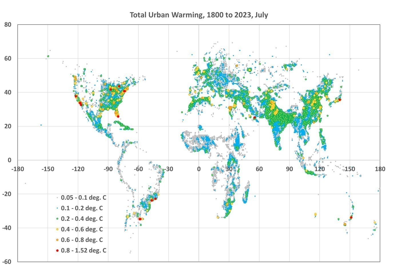
As an example of what one can do with the data, here is a global plot of the difference in July UHI warming between 1800 and 2023, where I have averaged the 1/12 deg spatial resolution data to 1/2 deg resolution for ease of plotting in Excel (I do not have a GIS system):
If I take the 100 locations with the largest amount of UHI warming between 1800 and 2023 and average their UHI temperatures together, I get the following:
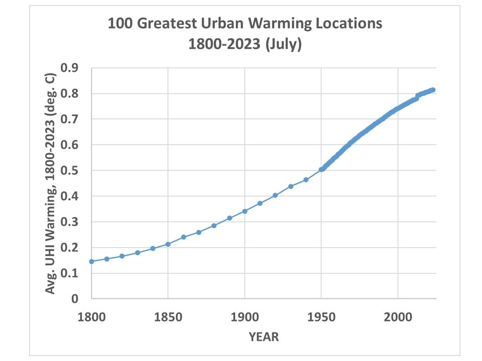
Note that by 1800 there was 0.15 deg. C of average warming across these 100 cities since some of them are very old and already had large population densities by 1800. Also, these 100 “locations” are after averaging 1/12 deg. to 1/2 degree resolution, so each location is an average of 36 original resolution gridpoints. My point is that these are *large* heavily-urbanized locations, and the temperature signals would be stronger if I had used the 100 greatest UHI locations at original resolution.
Again, to summarize, these UHI estimates are not based upon temperature information specific to the year in question, but upon population density information for that year. The temperature information, which is spatial (differences between nearby stations), comes from global GHCN station data between 1880 and 2023. I then apply the GHCN-derived spatial relationships between population density and air temperature during 1880-2023 to those population density estimates in any year. The monthly time resolution is to capture the average seasonal variation in the UHI effect in the GHCN data (typically stronger in summer than winter); the population data does not have monthly time resolution.
In most latitude bands and seasons, the relationship is strongly nonlinear, so the UHI effect does not scale linearly with population density. The UHI effect increases rather rapidly with population above wilderness conditions, then much more slowly in urban conditions.
It must be remembered that these gridpoint estimates are based upon the average statistical relationships derived across thousands of stations in latitude bands; it is unknown how accurate they are for specific cities and towns. I don’t know yet how finely I can regionalize these regression-based estimates of the UHI effect, it requires a large number (many thousands) of station pairs to get good statistical signals. I can do the U.S. separately since it has so many stations, but I did not do that here. For now, we will see how the seven latitude bands work.
I’m making the dataset publicly available since there is too much data for me to investigate by myself. One could, for example, examine the growth over time of the UHI effect in specific metro regions, such as Houston, and compare that to NOAA’s actual temperature measurements in Houston, to get an estimate of how much of the reported warming trend is due to the UHI effect. But you would have to download my data files (which are rather large, about 117 MB for a single month and year, a total of 125 GB of data for all years and months). The location of the files is:
https://www.nsstc.uah.edu/public/roy.spencer
You will be able to identify them by name.
The format is ASCII grid and is exactly the same as the HYDE version 3.3 population density files (available here) I used (ArcGIS format). Each file has six header records, then a grid of real numbers with dimension 4320 x 2160 (longitude x latitude, at 1/12 deg. resolution).
Time for Willis to get to work.


I think .6 to .8 should be light/bright purple rather than tan/brown/orange
A lot UHI effect near ocean/water and more than I thought in tropics/semi-tropics.
I think they think that yellow is a better transition to red.
Awesome work, Dr. Roy, and thanks so much for making the actual data available. I must investigate this, as time and the tides permit.
My very best to you and yours,
w.
Dr. Roy, a quick look at the data reveals this:
1941 12 04 08 52 41 -9999 315 10 -9999 -9999 -9999
1941 12 04 09 46 35 -9999 315 10 -9999 -9999 -9999
1941 12 04 10 41 30 -9999 315 10 -9999 -9999 -9999
A “Read Me” file explaining the meaning of each of the columns would be most welcome.
w.
Willis:
Those are the wrong files you found… look down the list. You want the .asc files, each labeled with a month and year.
Saturday morning I will remove the other files from that server since they are causing confusion.
-Roy
If I have correctly identified the “hotspots” (red), the winners are:
Sydney
Tokyo
Dubai
Rio de Janeiro
Sao Paulo
Buenos Aires
Miami
New York
Detroit
Chicago
San Diego
Los Angeles
San Francisco
I like how continental geography is obvious from the data points.
Basil
” I like how continental geography is obvious from the data points. ”
Though the graph below is no more than the raw output of a two-dimensional array, intentionally lacking any correction toward Earth’s spheroidal shape, maybe you’ll have some fun when looking at it:
https://drive.google.com/file/d/1AU6bR3flm7L6l7Yvm2GAwScJ6-VxbOdK/view
My comments
1. The effects of UHI are also significant during the day. Not just at night because higher surface temperatures over concrete and asphalt affect clouds.
2. Surface monitoring stations are too far away from power plants which discharge significant sensible and latent heat into the area.
3. Why isn’t the total rate of all energy use considered in the radiative balance?
Sam:
Energy use is trivial compared to radiative effects, except maybe in a traffic jam. It’s easy to demonstrate that.
-Roy
Are you sure about that?
If you divide the total energy use per year by the entire surface area of the earth that’s true. It comes out to less than 0.05 W/m
But if you divide the entire energy use in the USA 100 quadrillion BTU/year by a 1600 km x 1600 km area, you get 1.3 W/m. Most energy used in the USA is concentrated. This area would cover the area East of the Mississippi.
So while this may not be a factor in planetary heat balance it should impact regional climate.
https://www.eia.gov/nuclear/outages/
I got an email from NASA saying that anthropogenic evaporation doesn’t affect climate. That’s not what I’m seeing. When we shut down our coal plant in 2012, our lake temperature dropped, and the regional climate warmed a full 1C in ten years. Check Hartsville GISS. Our power plant data shows that it warmed during the winter months.
I think you’re doing great work BTW. IMO UHI effect is left out of global warming debate and it’s intentional.
Not sure if this is understood but when a power plant sends 1000 Giga Watts of electricity to a City, 2000 Giga Watts is sent to a heat sink. Only 1/3 of the total thermal energy is converted to electricity.
I meant megawatts. Not giga watts.
The Palo Verde Nuclear site has three nuclear units that generate 3×1400 Megawatt Electric. The total waste heat is approximately x 3 x 2590 Megawatts. This waste heat goes into the atmosphere via cooling towers. The total energy is 3 times the thermal energy generated by each unit which = 3 x 3990 MWth.
The nearest GISS station is 60 miles from this site. The total thermal load for a 60-mile radius is 0.27 W/sq.m
Since all three units came online by 1989, the temperature trend started warming and has warmed by 2 degrees C.
I can go on with other nuclear sites. My point is. I think there is something to be learned here. FYI Palo Verde elevation is 1000 feet so that might have something to do with warming.
We experienced cooling. Watts Bar experienced cooling.
Roy Spencer
Many thanks for the good work. I enjoy that you made your data publicly available.
I hope that, though increasingly disturbed by health problems, I’ll nonetheless have enough idle time in near future to go step by step into your data and process it.
It should not be so much more complicated than to generate latitude weighted, area gridded anomalies with annual cycle removal for GHCN daily or the combination of PSMSL tide gauge and SONEL GPS data.
*
” I used the ‘adjusted’ (homogenized, not ‘raw’) GHCN data because the UHI effect (curiously) is usually stronger in the adjusted data. ”
Still the same problem for me.
Why is this curious? I don’t see why it should be.
How do you manage to get rid of the effect of NOAA’s ‘Pairwise Homogenization Algorithm’ on the station data you analyze and compare yourself to other stations?
Menne’s PHA already modifies station data with its own strategy.
Thus, if not basing your analysis on the unadjusted variant of GHCN V4, you inevitably run into some PHA-generated bias(es).
*
The worst is when we read somewhere within NASA/GISTEMP’s web site that they recently gave up their homogenization software which processed NOAA’s raw data by its own, and now merely use their adjusted data! What a pity.
Bindion:
You misunderstand my use of the homogenized GHCN data. I do not use any trend information, only spatial differences between closely-spaced stations. In those comparisons, the homogenized data produce a somewhat stronger UHI signal than the raw data do. Thus, the homogenized data end up showing more UHI warming over time when the station-pair relationships are applied to the history of population density increases.
-Roy
Roy Spencer
I didn’t misunderstand you.
And I wasn’t talking about trends, how much they may differ between the two GHCN V4 variants.
What I was talking about was and still remains that when trying to look at UHI, I would never use such a highly adjusted time series when understanding that it was constructed out of adjusted, synthetic stations whose anomalies necessarily must contain information coming from nearby stations.
Did I understand Menne’s paper wrong?
binny…please refrain from bothering Roy with your trivial natterings. He’s a busy man doing real science.
Bindidon,
In my opinion, you have indeed misunderstood the homogenization method. Data from nearby stations are used to identify discontinuities. The series are cut at these points, but no values are added.
I would add that restoring the continuity of values for a particular station comes later, but is not problematic for quantifying UHI – quite the contrary.
The difference between the raw data and the homogenized data can be considered as a quantification of the UHI acting at short distances. The quantification made by Roy Spencer concerns UHI acting at long distances. To obtain the total UHI effect, we need to add these two components, which are of the same order of magnitude.
Robertson
You have long been known on this blog to discredit anyone, denigrate anyone whose work you don’t understand, or gullibly believe what contrarian blogs and people write about these people and their work.
*
This starts with your incredibly incompetent, endlessly repeated claim that NOAA only uses 1500 weather stations worldwide (last appearance: previous thread, November 3, 2023 at 7:19 p.m.), which is not only an outright lie, but also directly discredits the work of Roy Spencer himself, as he uses for research purposes the data of those ~27800 NOAA GHCN V4 stations that you claim only exist on paper or are never used.
*
It continues with, among other things
– Your denigration of centuries-old as well as recent astronomical results on the rotation of the Moon obtained by renowned scientists such as Cassini, Mayer, Lagrange, Laplace and their many contemporary successors, and your outright lies about Newton’s knowledge of and agreement with these results;
– Your infamous denigration of Einstein’s theories of relativity, which you don’t even understand a bit about;
– Your ridiculous claims that time doesn’t exist or that GPS technology doesn’t need relativistic corrections, etc. The list is long.
*
If there’s anyone who should refrain from vilely abusing this blog’s freedom of expression, it’s you, Robertson.
But unfortunately people like you never stop spreading their disgusting lies.
binny…”but also directly discredits the work of Roy Spencer himself, as he uses for research purposes the data of those ~27800 NOAA GHCN V4 stations that you claim only exist on paper or are never used.y…”
***
Not so. I have never disputed that NOAA has over a 100,000 surface stations available in the GHCN database. I have only pointed to the fact that NOAA themselves, on their own site, admitted to slashing ‘global’ surface stations from 6000 to less than 1500.
They are not the only ones. Gavin Schmidt at NASA GISS has admitted in the past that they lack the resources to check out such a number of stations for accuracy. So, they too limit the number of stations they use for their work. Ofcourse, GIS gets their data each month from NOAA therefore they too must be limited to less than 1500.
From NOAA…
“Why is NOAA using fewer weather stations to measure surface temperature around the globe from 6,000 to less than 1,500?
The physical number of weather stations has shrunk as modern technology improved and some of the older outposts were no longer accessible in real time”.
https://web.archive.org/web/20150410045648/http://www.noaa.gov/features/02_monitoring/weather_stations.html
So, NOAA is trying to tell us that, as telemetry has improved, so remote stations can report more easily, they have slashed the number of reporting stations from 6000 to less than 1500 because they are no longer accessible.
I have heard double-talk in my time but that takes the cake. In another part of the article they claim that, although the number of stations has been slashed, the database has grown. It takes a special kind of addled mind to accept such tripe.
Robertson will NEVER stop ly~ing and mis~representing anything he dislikes because it does not match his ego~maniacal, patho~logical narrative.
How is it possible to write such an incredible trash on a blog owned by a scientist who uses exactly that data which a 100% ignoramus claims not to exist?
How is it possible to be so du~mb, so stubborn, so opinionated?
*
The NOAA communication that Robertson is talking about appeared on the Wayback Machine in 2010 for the first time.
What the NOAA people discussed on that page is what happened in GHCN V2 between 2007 and 2009, as a big station inventory change happened.
*
It is easy to find in the Wayback Machine the oldest crawled revision of GHCN V2’s successor GHCN V3, which was, oh miracle, stored together with the directory above:
https://tinyurl.com/Wayback-GHCN-V3
Gunzipping the file gives you a directory with the two usual ‘.inv’ and ‘.dat’ files (station list resp. data), both dated 2013, Oct 25.
A wc on the station list (‘ghcnm.tavg.v3.2.2.20131025.qcu.inv’)
gives 7280 stations, exactly the same amount as in 2019, as V3 was shut down because it was replaced by V4 which is currently used by Roy Spencer (and, among many many others, I myself).
*
I never used GHCN V2, but it was easy to find tracks of the series’ entire directory and, oh miracle again, of the contents of the station list itself, named in V2 ‘v2.temperature.inv’ (last successful crawl on 2005, Nov 29):
https://tinyurl.com/Wayback-GHCN-V2
When downloading the file, you see that it contains… 7280 stations, which however build a set differing from that in V3′ 2013 station list (which, in 2011, still contained only… 7278 stations – he he, some might understand what I mean here).
*
Most of Robertson’s misinformation comes from the contrarian blog ‘chiefio.wordpress.com’ managed by a guy named ‘E. M. Smith’.
Smith-chiefio’s most brazen head posts were apparently written in the middle of the GHCN V2 station set reorganization process, what led him to claim that
– only one GHCN station remained in the Canadian Arctic;
– only four (not: three) GHCN stations remained in California.
He hardly could have shown a higher niveau of incompetence.
And, no wonder that similarly incompetent people like Robertson of course gullibly follow Smith-chiefio as if he was the weather station pope in person.
*
I checked both V2’s and V3’s station lists, and you can be sure that there were (from 2005 till 2019) and are currently far far more California stations then stoopidly claimed by Smith-chiefio (namely about 55 in V2, and about 115 in V3).
Currently, there are about 580 California stations in V4, and exactly 619 in GHCN daily (all GHCN daily stations for US & Canada have a state attribute).
*
There are 3644 Canadian stations in GHCN V4 (847 in V3); starting with
CA002100163 60.0000 -136.7667 836.0 BLANCHARD_RIVER
and ending with
CA002400300 82.5167 -62.2833 30.0 ALERT
232 of them are in the Canadian Arctic (there were 100 at or north of 60N in V3).
*
Who believes Robertson’s endlessly repeated trash about everything 100% deserves it.
phi
” Data from nearby stations are used to identify discontinuities. The series are cut at these points, but no values are added. ”
Ici, vous discutez du sexe des anges.
I never told about any value being added, I said that ” anomalies necessarily must contain information coming from nearby stations. ”
I does not matter to me whether the data of nearby stations is included into that of the ‘homogenized’ stations, or the data of these is partly suppressed wherever nearby stations indicate their discontinuity.
Fact is that this homogenization has a huge influence on the time series containing UHI biases in either variant, as comparisons of adjusted to unadjusted data show.
1. CONUS 1900-2023
https://drive.google.com/file/d/1y2lzVrYU8dBablqb4cuGyBL6UvSaegv_/view
2. Globe 1900-2023
https://drive.google.com/file/d/1x4o2eqXYXkPb10cNJPEEDq2zJ6BqwJJ3/view
*
Any quantification of UHI based on homogenized time series can be influenced by the homogenization process itself.
Thus, if I were a reviewer, I would ask the persons submitting the paper
” Why don’t you start with the unadjusted data, showing UHI effects present in the raw variant of the time series, and then move on with the adjusted data, and compare the results obtained in the two steps? ”
*
Review processes are, it seems, so unpredictable that one should perhaps smooth the path to the paper’s success in advance.
Mr Spencer wrote above:
” Thus, the homogenized data end up showing more UHI warming over time when the station-pair relationships are applied to the history of population density increases. ”
I pretty good imagine the reviewer asking
” Yeah sure. But to what is this ‘more UHI warming’ basically due to? Can you exclude any influence due to homogenization processes? ”
C’est tout ce que je voulais indiquer, phi… Ni plus ni moins.
As homogenization fundamentally consists of dividing the series into homogeneous sections, the effective value of the correction can only be determined on the basis of long raw series. It follows that the effective correction for GHCN V4 is actually 0.5 C since 1940.
Our paper DOES include calculations using raw data, which we compare to results using homogenized data. We do those comparisons in several historical periods, 1880-1920, 1930-1950, 1960-1970, 1980-1990, 2000-2010, and 2015.
phi…re homogenization. One of the problems with such a method is the ability to cherry pick the surrounding areal temperatures to which interpolation and homogenization is applied to derive a synthesized temperature for another region..
For example, at one time, there were no surface stations in Bolivia, which tends to be a country of higher elevation hence cooler temperatures. The powers that be selected temperatures from surrounding countries that were lower altitude and warmer to average a temperature for Bolivia, which ended up with a much warmer temperature than it should be.
Same in California. Despite the protestations of Binny, NOAA uses only 3 surface stations in California, all near the ocean. That excludes areas inland like the Sierra Nevada mountains, which are obviously cooler, especially at night.
I don’t see thermometers at the peaks of Mt. Everest or any other mountain in the region where many peaks are above 8000 metres, hence much cooler. Seems to me, if you are going to declare an average temperature for the planet, the coldest regions should be included in the analysis.
Roy Spencer
” Our paper DOES include calculations using raw data, which we compare to results using homogenized data. ”
Thank you.
By the way, I would not like to be misunderstood when insisting on the use of unadjusted data.
Because exclusively relying on it can create biases as well when you ignore the effects of discontinuities, which can arise for example when in the past manual thermometer readings were wrong over longer periods, what had to be corrected by using the data of very nearby stations.
I have always missed an intermediate stage of ‘corrected’ between ‘unadjusted’ and ‘adjusted’.
phi… re homogenization (part 2)
” For example, at one time, there were no surface stations in Bolivia, which tends to be a country of higher elevation hence cooler temperatures. The powers that be selected temperatures from surrounding countries that were lower altitude and warmer to average a temperature for Bolivia, which ended up with a much warmer temperature than it should be. ”
*
Hmmmh. Always the same source:
https://chiefio.wordpress.com/2010/01/08/ghcn-gistemp-interactions-the-bolivia-effect/
” Alright Already, what is this Bolivia Effect? ”
*
Years ago, I invested some idle time into that, and found 32 stations surrounding Bolivia by up to 500 km in Argentina, Brazil, Chile and Paraguay:
https://drive.google.com/file/d/125hoAWPb-C9t1X4WCUuBrQxBBvaxowap/view
Sans commentaire.
phi
I come back to your claim:
” Data from nearby stations are used to identify discontinuities. The series are cut at these points, but no values are added. ”
Where does your claim exactly come from?
At the time I used GHCN V3, I made quite different experiences.
*
The most typical of these was when a Czech ‘skep~tic’ commenter at WUWT had heavy doubts about the correctness of the adjusted data for one of his ‘home’ stations he saw in GISTEMP’s V3 station data at that time.
He thought the data was fudged. { But… probably only because the correction’s result gave a higher trend, he he. }
*
In the graph you see that the adjusted data replaces the unadjusted variant:
https://drive.google.com/file/d/1klpZ0hdJ10XEHW9DIsBBU9-ixvREKiZT/view
which is no simply cut off.
Menne M. J. et all. (2018) : The Global Historical Climatology Network Monthly Temperature Dataset, Version 4
Identifying a jump causes a break in the series without removing any value but there is a loss of information because the two sections become floating relative to each other.
There is no other alteration. The incidental reconstruction of series adjusted on this basis has no influence on the regional or global evolution because it is done using only the values already available.
Any break has an effect on the trend, including those carried out before the homogenization phase.
The effect of the method can only be quantified using a technique that preserves the long-term trend.
Correct, thx!
I had downloaded the paper but hadn’t read it yet, my bad; so I was still in ‘V3 mode’ (I don’t use V4 because unlike V3 and daily, it lacks Tmin/Tmax).
Hmm,
clicking on one of the files;
https://www.nsstc.uah.edu/public/roy.spencer/Tuhi_APR_1830AD.asc
gives;
“Forbidden
You don’t have permission to access this resource.”
**********************
Ken:
You are correct, I get the same message, despite this being a location for public access of data. I will have someone fix it on Monday.
-Roy
Since most large, growing cities that manifested the strongest UHI during the last century are located in the northern hemisphere, it seems inadvisable to take July as representative. That summer month is naturally the least variable in that hemisphere and there’s practically no artificial, fuel-generated winter heating. It would be more revealing to show January results instead.
UHI effects are strongest in the summer and weakest in the winter, generally speaking. The UHI effect is mostly due to solar energy, not waste heat, acting on impervious surfaces that have higher heat storage capabilities than their natural counterparts.
Roy,
I think you are mistaken in invoking an inertial source at the UHI. Inertia can reduce the difference between maximums and minimums but does not a priori modify the average temperature. The simple energy balance seems much more relevant to me with the effects of urban drainage and energy consumption.
Phi, putting some numbers to the problem…. I use Portsea island in the uk, because it is densely populated and has a very clear boundary.
Population density 5100 people / km2
Area per person 196m2
Heat output per person 100 watts
Or 0.5 w/m2
Energy used per person in the uk, 30,098kwh/annum
Or 3.43kw average
Or 17.5 w/m2
Verse
Solar insolation 0.49 kwh/m2/day December, average 20watts/m2
Solar insolation 4.7 kwh/m2/day July, average 195 watts/m2
But the built environment would not absorb/store all of that energy…..
So just ballpark numbers. In the winter a person’s heat & energy use would have a larger affect on the uhi that during the summer months.
*numbers are from various sources, so just ballpark at best.
My values for annual energy balances in central Europe in W/m2:
Rural Urban
Sun. 135 135
Evap. -37 -7
Energ. – 17
Tot. 98 145
So there is about 50% more power for sensible heat in an urban environment.
Evaporation primarily affects Tmax and summer while energy is probably more sensitive in winter and for Tmin.
An inertial effect could be added to this but it involves taking into account the variation in the day/night weather regime. A consequence of this variation in regime is that the method used by Roy Spencer probably cannot correctly capture the effect of evaporation which is rather short-range (rising air).
It would be very interesting if Roy Spencer did the exercise for a winter month.
I add that the in-depth study of temperature series is not the only way to demonstrate and evaluate the UHI. The use of temperature proxies (including UAH LT) makes it possible to evaluate it globally. Quantitatively and very roughly, current effective temperatures are quite close to those of the 1940s. Practically, anything that exceeds these values today is due to UHI and inappropriate processing of temperature series.
phi
” The use of temperature proxies (including UAH LT) makes it possible to evaluate it globally. ”
Do you mean something like this, for example?
https://drive.google.com/file/d/1ZGRLXFt9E2-kNxE7Mwuj9le7kCYKchRF/view
Trends in C / decade
– UAH: 0.19 +- 0.008
– V4: 0.21 +- 0.006
Could be worse.
Of course: this is just a trivial layman comparison which needs verification & validation at grid cell level.
*
Ooooh! Me thinks the man with the big feet and the pea brain might come over and write below:
” He has once more the temerity to show UAH and NOAA in lock-step !! ”
Woooaah! I think with something like that I’m ready for Punishment Park.
*
” Quantitatively and very roughly, current effective temperatures are quite close to those of the 1940s. ”
https://drive.google.com/file/d/1ZmMgjpLEcEkG8uinoR1L3NSVLeKPJHk2/view
If you say so, if you say so…
Some accurate data for a valuable contradiction?
I mentioned using UAH LT as a proxy for surface temperature and not as directly comparable data. A proxy must be calibrated. In the particular case there is a physically demonstrated relationship between the two. The increase in absolute humidity with temperature amplifies temperature variations in the lower troposphere. If there is doubt about long-term trends, the recommended method for any proxy is to evaluate the ratio of the two variables based on the detrended series.
https://www.zupimages.net/up/22/16/804k.png
Roy,
My experience is that a section of bitumen (or any other inert object) roadway is exactly the same temperature as a piece of foil covered insulation next to it, just before sunrise. Heat does not get “stored” overnight – as the operators of solar generating plants like Ivanpah have found out to their cost.
Deserts which get extremely hot during the day, also get extremely cold during the night, to the point where ice can be manufactured using basic knowledge going back thousands of years.
Maybe you could expand on on “UHI is mostly due to solar energy”, and explain what “mostly” means in numerical terms, as well as how fixed “solar energy” results in higher “average” temperatures.
It all seems a bit vague. You obviously think that I am mistaken, but if you feel like alleviating my lack of knowledge, supported by experimental results, of course, I would be grateful.
Or you could try patronising sarcasm, appealing to your own authority. Banning dissent?
As Feynman wrote “It doesn’t matter how beautiful your theory is, it doesn’t matter how smart you are. If it doesn’t agree with experiment, it’s wrong.”
I appreciate your research into the numbers. Maybe your ideas for the reasons behind them don’t stand up to scrutiny, is all I’m saying. Blithely saying that the UHI is “mostly” due to “solar energy” is like saying that heatwaves and cold snaps, floods and droughts, are due to carbon pollution.
Let’s remember that UHI is most clearly revealed by the pair-wise relationship between validated (NOT homogenized) major urban station records and those from neighboring small-towns and rural locations. Amongst hundreds of such century-long comparisons that I’ve made throughout the globe, I don’t recall encountering any that show consistently stronger discrepancies in summer.
No doubt impervious urban surfaces can heat up more than vegetation or soil, but the air temperature at the 1.5m elevation of station thermometers doesn’t necessarily follow. Evaporation and moist convection, not radiation, are the principal means of surface heat transfer on an aqueous planet with a semi-absorbent atmosphere.
Roy…good for you. It’s heartening that someone like you (and John) have the interest and integrity to pursue this kind of science.
When I started college, computer input was on 80 column Hollerith cards without printing thereon. Young readers can find an explanation on the Web.
The size of your data files swamps my ageing mind. Likely they would swamp my DSL connection too!
Thanks for your contributions all these many years.
Dr Roy Spencer, is the data compressed? You might be able to compress it down to 6GB.
No, the files are not compressed. You are right, it would probably be a good idea to provide compressed files.
Indeed, Mr Spencer – especially for those of your readers who have to live with poor 16 Mbit/sec…
What have we learned?
Cities are hotter than surrounding suburbs and rural areas, but a lot of people choose to live there, so people must like hot cities.
Whatever the actual UHI increase is included in the global average temperature, it does not affect the 71% of our planet’s surface that are oceans.
No matter how accurate the historical global average temperature data are, the leftists will predict a coming climate crisis, as they have done since the 1979 Charney Report.
Someday leftists will claim climate change will kill your dog … before it gets you.
44 years after the Charney Report in 1979, no one knows exactly how much of the post-1975 global warming was caused by humans, or more specifically by CO2.’
A century of environmental predictions of doom have been 100% wrong.
The only correct climate prediction in the history of the world was my own, from 1997: “The climate will get warmer unless it gets colder”.
I’ve been thinking about the issue of people choosing to live where it’s warmer. In the U.S., people migrate southward, from where it’s cooler to where it’s warmer. And globally, 50% of humanity now lives in urban areas. That fraction is expected to be 2/3 by 2045. Do people realize most of the warming they experience is through choice? You might object, they have to for economic reasons… which is part of my point… economics trumps climate change.
The future is hard to predict, I try to limit it, to a decade.
A lot could change in a decade.
Recently people are saying cities are dying. And it doesn’t seem having more homeless is helping. Office space has high vacancy apparently. One thing cities have is major or international airports,
but there seems to effort to destroy the airline pilot’s business- planes falling out to sky, also doesn’t help.
It seems the big thing within a decade will the beginning effects of lower population in large areas of world, particular China, Japan, and South Korea. Though for most of world’s population it’s effects will take more than a decade.
It seems we will know within a decade whether or not the lunar polar region has mineable water. If not really, is the result, not much effect within 10 years, but “oh my God! How could there be so much water”. It could quite a bit of an effect.
And in couple of years, should have some idea of whether or how well, Starship works. Also within couple years a lot could change other just having to do with Starship. So, does Blue Orgin, finally stop preceding cautiously, will new CEO, change things within 6 months.
Anyways, if parties are mining the Moon within 10 years, it seems to me we also have ocean settlements. And ocean settlement might make coastal cities, more attractive.
One aspect of starship is potential ability to replace airline travel, and such suborbital travel will be done from ocean point to ocean point to lessen sonic booms effects. And could also related growing aspect of India and Africa- in terms US, the travel time in made rather short with suborbital travel.
It seems given India will make a lot progress in 10 years- though conflicts within Africa may continue to inhibit as much progress- it might more of a couple decades type of thing.
GB,
Great! Where’s the stock market going to be next month?
Last 5 business days it when up by 1000 and was 34,061.
In month +/- 1000 of 34,000.
If you could predict more than year, you would be rich.
I predict the stock market will go up,
unless it goes down.
Not trying to get a laugh here … but people carry more blubber (scientific term for fat) insulation these days, so they FEEL warmer than pre-1975 global warming, when obesity was less common.
In summary, people tend to live in cities or near cities, tend to move south rather than north, and tend to vacation in warm or hot areas in the warmer months of the year.
Anecdotal evidence shows people preferred warm centuries over cold centuries, long before AC was invented.
We are living in a gradually warming trend during an interglacial period. That seems like an ideal climate for people and animals on our planet. We should be celebrating the current climate.
Here in SE Michigan, our winters are warmer, with less snow, than in the 1970s. Last summer was unusually cool with the most rain of any summer since the 1970s. We LOVE our climate change here, based on local conditions. We could not care less about a global average temperature that not one person lives in.
My predictions are not always 100% accurate. In 2020, I predicted the US would be invaded by aliens. That prediction was half right. We were invaded by aliens from South America. However, i had predicted an invasion of aliens from the planet Uranus.
roy…you can see it here in Vancouver, Canada, and the relocation is not only due to temperatures, it’s due to scenery and recreational facilities as well.
Thousands of people in Canada, native to interior Prairie provinces, relocate to Vancouver due to its warmer climate. However, it has a lot to do with economics and livability. There is simply more work around Vancouver for young people and more to do entertainment-wise.
The surprising part is that people who have lived in Alberta all their lives relocate to south-central areas in British Columbia for retirement. So, they are relocating from a colder area to a not-as-cold region, but it’s still cold in winter. Also, hey are not plagued by tornadoes or severe thunderstorms, s only the Prairie provinces can experience them in Canada.
I have lifelong friends from the Canadian Prairies who moved here at a young age and never returned.
Why Is the 1st Satellite Observation Sidelined?
https://www.youtube.com/watch?v=GtgaXD0Rr9g
Gold has an emissivity of
ε = 0,02 !!!
–
According to generally accepted science, a golden surface without-atmosphere Earth, with the same Albedo (a ~0,3) would develop an equilibrium temperature of
Te = 678K !!! (405 oC)
–
https://www.cristos-vournas.com
Doctor Spencer, in addition to the heat input of mankind, I see an important factor that has not been taken into account: //German Weather Service//In total, the year 2022 brought an average of 2024.1 hours of sunshine in Germany. This results in a significant surplus compared to the multi-year average annual total for the period from 1991 to 2020 (359.3 hours or +21.6 %). Compared to the international climatological reference period 1961-1990, there is a surplus of 480.1 hours or +31.1 %.
Global radiation 1983-2022 in Germany/yearly totals, decade average and trend (+3.61 kWh/square metre per year)
Source: German Weather Service.(dwd.de)
Klaus
I live in Germany, am interested in processing various weather/climate data and downloaded the hourly data from the DWD weather station last month at the latest.
If you perform a descending sort of the yearly average of that data in absolute form, you will indeed see 2022 on top of the list, topping 1943 by just 0.01 C:
2022 9.43 (C)
1943 9.42
2020 9.34
2014 9.34
2018 9.26
2019 9.14
1946 9.14
2015 8.90
1949 8.70
2016 8.61
But is that due to solar radiation?
A monthly output shows, similarly sorted:
2006 7 20.02 (C)
1994 7 19.33
1946 7 19.30
1947 8 18.93
2003 8 18.87
1947 7 18.82
2010 7 18.74
1943 8 18.72
1941 7 18.72
2022 8 18.65
2022 appears in 10th position within the list of months with usually most sunshine.
*
When switching to anomalies (aka depar~tures from a mean with annual cycle removal), with as reference period 1981-2010:
2015 12 5.22 (C)
1947 9 5.05
1990 2 4.92
1946 4 4.57
2020 2 4.40
2007 1 4.12
2019 6 3.97
1946 5 3.95
2018 4 3.91
1943 2 3.89
we see that as so often, the increase is due more to months outside of the summer, and even
2022 10 3.53
appears at position 23 in the sort.
*
What bothers me is less the current increase in solar radiation in Germany (possibly due to the extreme decline in air traffic in Europe in 2020/2021, which resulted in significantly lower injec~tion of H2O/CO2 at tropo~pause altitudes), but rather the increase in the temperature trend here since 2010, in C/decade:
– 1941-2023: 0.18 +- 0.02
– 1979-2023: 0.52 +- 0.05
– 2000-2023: 0.58 +- 0.10
– 2010-2023: 1.15 +- 0.30
This is exactly the opposite of what is happening in Northern CONUS for example.
*
Source
https://tinyurl.com/DWD-hourly-data
(idem ‘recent’)
https://tinyurl.com/DWD-anoms-1941-2023
https://tinyurl.com/DWD-anoms-2010-2023
Thanks Bindidon , for this valuable information. but there must be a correlation between cloud cover and solar radiation. Please take a look at this plot // https://www.dwd.de/DE/leistungen/rcccm/int/rcccm_int_cfc.html
Here you can see the annual variation of cloud cover from 1979-2023.
Manns “Dirty Laundry”
“As the date approached for the Mann-Steyn/Simberg libel trial, Ive been reviewing my files on MBH98 and MBH99. Its about 15 years since I last looked at these issues”
https://climateaudit.org/2023/11/07/manns-dirty-laundry/
Thanks Bindidon , for this valuable information. but there must be a correlation between cloud cover and solar radiation. Please take a look at this plot // https://www.dwd.de/DE/leistungen/rcccm/int/rcccm_int_cfc.html
Here you can see the annual variation of cloud cover from 1979-2023.
Klaus
” … but there must be a correlation between cloud cover and solar radiation. ”
Thanks / Danke / Merci…
I’ll have a look at that (which imho seems evident: more clouds -> less solar, but insolation of cloud tops should have some consequences too).
Bindidon
Yes, the clouds also hold back the heat radiation from the earth’s surface. but if they hold back more radiation from the sun than radiation from the earth, it gets colder. – Because the earth has no heat energy source of its own, apart from a few volcanoes and the negligible heat input of mankind in this case, it will be the task of future generations to investigate these processes in more detail.
phi
” I mentioned using UAH LT as a proxy for surface temperature and not as directly comparable data.
A proxy must be calibrated.
In the particular case there is a physically demonstrated relationship between the two. The increase in absolute humidity with temperature amplifies temperature variations in the lower troposphere.
If there is doubt about long-term trends, the recommended method for any proxy is to evaluate the ratio of the two variables based on the detrended series.
https://www.zupimages.net/up/22/16/804k.png ”
I know of your old graphs.
It’s always the same: your by no means unbiased confusion of “LT” with “UAH”.
You only need to look closely at this simple WFT chart
https://tinyurl.com/UAH-vs-RSS-vs-GIS-vs-Had
to see that UAH is only considered a better proxy than RSS for ideological, pseudo-skeptical reasons.
If you take the trend out of both:
https://drive.google.com/file/d/1NVZ2tQgazEr-qPkjabC3um9cKeGgshxT/view
the question is why one should be better than the other because simply detrending is not enough: you still have to explain the remaining difference.
Both are equally inappropriate: like for the surface, each atmospheric time series has its own views on what is happening.
1. As seen above, homogenization of surface data does not preserve long-term trends.
2. UAH LT trends were recently confirmed by NOAA’s STAR LT series : 0.135 K/decade since 1979 (https://www.star.nesdis.noaa.gov/smcd/emb/mscat/).
3. UAH calibrated for the surface is compatible with surface proxies (dendro, gladier, ocean levels, etc.) which neither RSS nor surface indices are.
I had to interrupt the little job last night and reconstructed the baselines destroyed by the detrending procedure.
The graph was updated below the Drive link:
https://drive.google.com/file/d/1NVZ2tQgazEr-qPkjabC3um9cKeGgshxT/view
and here you see that the difference between UAH’s and RSS’s detrended series, when correctly displaced wrt the same reference period (1991-2020), is minimal.
Both Savitzky-Golay smoothings are kept within [-0.14, +0.11].
The same is visible for a graph including GISS LOTI:
https://drive.google.com/file/d/1O3VftEiJPC7okzKQwsC6bXH0iPRKw_l4/view
I don’t see any technical let alone scientific reason to use UAH as ‘calibration’ tool for anything.
*
” If there is doubt about long-term trends, the recommended method for any proxy is to evaluate the ratio of the two variables based on the detrended series. ”
Are you really serious, phi? Such a trivial evaluation for such a complex task? This sounds to me like the ball-on-a-string method proving the absence of a lunar spin.
You should give us a link to the source from which you obtained the info.
*
Moreover, when you write:
” UAH calibrated for the surface is compatible with surface proxies (dendro, gla[c]ier, ocean levels, etc.) ”
I’d like to see a valuable source confirming that as well, at least for the sea levels.
When I compare the undetrended data for sea levels (tide gauges plus sat altimetry) to UAH LT
https://drive.google.com/file/d/1oCgDT8P1YGtm7cdDfCd2dKjy7EYgd1tR/view
I would enjoy you showing me
– how good sea levels work as ‘surface proxies’ for the period 1900-2022
https://drive.google.com/file/d/1YkJvOTEqJbecLFHUBpGpjChWnzA-u5xX/view
– what you understand with this ‘compatibility’.
I begin to doubt you would be using UAH for your ‘calibration’ purposes if Spencer/Christy hadn’t moved from 5.6 to 6.0 and Mears/Wentz from RSS 3.3 to 4.0, respectively.
“I dont see any technical let alone scientific reason to use UAH as calibration tool for anything.”
I don’t use UAH as a calibration tool, I calibrate UAH with the standard tool. I use UAH as just one benchmark to assess the long-term trend in surface temperatures. This is because the method of constructing surface indices does not preserve this long-term trend.
“Such a trivial evaluation for such a complex task?”
In the case of TLTs, the essential physical link is known and the relationship can legitimately be assumed to be linear in the domain of values concerned. This is confirmed by the excellent correlation of the curves in the fourth graph of the board.
For the ocean level, the relationship is complex but it is close to linearity between the rate of sea level rise and the temperature. The variation in rate essentially depends on the melting of continental ice which is in a linear relationship with global temperature. According to tide gauges, the current rate of level rise is close to that of the 1940s (see for example Dangendorf 2017 fig. 1b).
” … but it is close to linearity between the rate of sea level rise and the temperature. ”
Yeah. When comparing the 180-month cascaded triple running means of two time series, they inevitably become sooner or later similar.
*
” … (see for example Dangendorf 2017 fig. 1b). ”
I used Dangendorf’s data as ‘proxy’ for a V&V of my own evaluation.
But… as a good ‘skep~tic’, you might doubt its correctness and accuracy.
*
” According to tide gauges, the current rate of level rise is close to that of the 1940s… ”
Typical cherry-picking of a single, short period – the tree hiding the forest.
Here is a chart showing, from the period 1903-1912 till the period 2013-2022, the 10-year running trends, computed out of Dangendorf’s PSMSL evaluation till 2015, and out of NOAA’s sat altimetry later on:
https://drive.google.com/file/d/12MHMaLzSV0NX1f45Xt_cMjuz4iE4mrZh/view
As you can see, your cherry-picking is 100% wrong: the highest 10-year trend ‘in the 1940s’ was 1933-1942 with 2.2 mm/yr.
Look at the right end of the graph. Dangendorf’s data ends with a 10-year trend for 2006-2015 of 3.4 mm/yr, and the sat altimetry finally shows for 2013-2022 4.0 mm/yr.
Interesting: the trend comparison Dangendorf vs. NOAA sat altimetry for their common period (1993-2015): 2.8 vs. 2.7 mm/yr.
*
Imho also of interest is how the trends moved from 1900-2015 till 1995-2015.
Here are the 5-year consecutive trends for various evaluations of PSMSL gauges and SONEL GPS velocities – Dangendorf, Frederikse, Foster, NOAA, Bin(didon):
https://drive.google.com/file/d/1dvz115qfZXH95nkoIXF091JJsaasaAEn/view
*
By the way: Dangendorf and his team were heavily criticized and discredited because of their paper’s title mentioning the ‘forbidden word’ acceleration.
But… ‘by accident’ of course, the data of all PSMSL evaluations shown above tells the same for the aforementioned ‘since 1960’:
https://drive.google.com/file/d/1ZAx1FAHRFdr27zlzdKE2XyckdPBbASA8/view
Bindidon,
I’ve seen quite a few forged charts, yours deserves a special mention.
1. Your tide gauge curve is shifted towards the past by 6 years.
2. Your last value represented is 2006, so in reality 2006 + 6 = 2012 which corresponds to the last year available in the data. Smoothing over 10 years means that the last 5 years have arbitrary values. There is no more usable data in your work after 2007 (2001 in your graph).
3. The curve closest to the tide gauge data is the red one (GIA only). Successive corrections which always go in the same direction is the great specialty of climatology.
4. Satellite data are not shifted towards the past. There is therefore a gap of 6 years between the two series. The apparent agreement between satellite and tide gauges is only the result of your cumulative errors.
Conclusions:
– Your graph constitutes a characterized manipulation of data.
– Your 3.4 mm per year at the end of the series makes absolutely no sense. Your criticisms are therefore unfounded.
– Surface temperature indices are incompatible with changes in sea level.
– An evaluation of the long-term trend based on UAH LT makes it possible to obtain a temperature series consistent with the behavior of the oceans.
phi
I didn’t expect any valuable answer from your side, and… it shows.
1. Ive seen quite a few forged charts, yours deserves a special mention. ”
You are a brazen boy, aren’t you?
You make a long series of strange allegations, all without any proof – as usual for pseudo-skep~tical persons.
What for a nonsense are you telling us here, phi?
You manifestly were not even able to generate a chart out of a display of available final data from other sources, let alone one out of an own processing of raw data.
Otherwise, you very certainly would have posted a link to that graph.
So the only option left to you is discrediting and denigrating, isn’t it?
*
2. ” Your tide gauge curve is shifted towards the past by 6 years. ”
So?
2.1 Which graph do you mean? This one?
https://drive.google.com/file/d/1YkJvOTEqJbecLFHUBpGpjChWnzA-u5xX/view
*
2.2 Which tide gauge curve do you mean? The green one?
The data behind the green curve starts in 1900 and ends in 2022!
Why don’t you show exactly what you criticize?
*
3. ” Your last value represented is 2006, so in reality 2006 + 6 = 2012 which corresponds to the last year available in the data. ”
” There is no more usable data in your work after 2007 (2001 in your graph). ”
Again: Which chart and which curve in it do you mean? What does stop where in 2006 resp. 2001?
Where do you get that confused nonsense from?
*
4. ” The curve closest to the tide gauge data is the red one (GIA only). Successive corrections which always go in the same direction is the great specialty of climatology. ”
That becomes now really ridiculous, and furthermore disgusting.
Which tide gauge data do you exactly mean?
Where is your link to a graph showing that?
You don’t know anything of what you are telling about here: the evaluations published by Dangendorf et al., Frderikse et al., Grant Foster and myself all were made such that the tide gauge data was wherever possible corrected by the vertical land velocity data provided by SONEL. (About NOAA’s gauge data I know nothing.)
My evaluation was made such that, as requested by professionals, the data of only those PSMSL gauges with a GPS station located sufficiently in their near was used.
*
5. ” Satellite data are not shifted towards the past. There is therefore a gap of 6 years between the two series. ”
What exactly do you mean with that?
– I have PSMSL’s tide gauge data on disk till end of 2022 (no problem to download 2023 if necessary)
and
– Sat data starts in 1993.
Don’t you know that?
Where is your 6-year gap?
* ” The apparent agreement between satellite and tide gauges is only the result of your cumulative errors. ”
You do not seem to be able to produce anything else than cheap, superficial and above all unproven insinuations.
*
6. Your so-called ‘conclusions’ show exactly as much competence as the text preceding them. Nothing unsual for people trying to appear as very knowledgeable by writing long comments doubting about everything, but who in fact lack the ability to contradict.
It is also typical for people like you that you not only omit to back up your criticism technically let alone scientifically, but don’t even bother to include a link to the graphics you criticize so that one knows what exactly what in them you criticize, and for which valuable reason.
If you had any REAL technical skill and scientific knowledge, you would have posted something quite different.
*
7. Finally, a little hint.
https://drive.google.com/file/d/1qQ_sIIQNkCF3PDOZvCS4VJnFySP8WrOu/view
Maybe you think a bit about it.
*
A part chez le posteur Robertson, je n'ai jamais vu pareil mélange d'incompétence et d'une malhonnêteté qui frise le mensonge intentionnel.
Spare us your blabla, insinuations and off-topic . Your graph is obviously this one: https://drive.google.com/file/d/12MHMaLzSV0NX1f45Xt_cMjuz4iE4mrZh/view
phi
You wrote on November 15, 2023 at 5:22 AM:
” Your tide gauge curve is shifted towards the past by 6 years.
2. Your last value represented is 2006, so in reality 2006 + 6 = 2012 which corresponds to the last year available in the data. Smoothing over 10 years means that the last 5 years have arbitrary values. There is no more usable data in your work after 2007 (2001 in your graph). ”
And now, on November 21, 2023 at 5:40 AM you write
” Your graph is obviously this one:
https://drive.google.com/file/d/12MHMaLzSV0NX1f45Xt_cMjuz4iE4mrZh/view ”
*
Are you serious? This is BY NO MEANS a tide gauge curve, phi.
This is a couple of 10 year running trend curves over Dangendorf’s tide gauge resp. NOAA’s sat altim data,
– starting, over Dangendorf’s data, with the trend for 1903-1912 and ending with that for 2006-2015;
– starting, over NOAA’s sat altim data, with the trend for 1993-2002 and ending with that for 2013-2020.
The resulting curve was intended to show you how wrong you are with you claim that the 1940s are at the same level as today.
Apparently, you don’t seem to know what is a running trend, used to show how trends move over short periods of time series.
*
FYI, here are the tide gauge and sat altim curves you naively thought to have detected in the running trend graph you mentioned:
https://drive.google.com/file/d/1xkdM6bd47s2WWraL2I6p2Nmz3g70JzNL/view
It shows the agreement of gauge and altimetry measurements
– when the tide gauge time series are displaced by the vertical movement velocity (positive for isostatic rebound, negative for subsidence) provided by one or more GPS stations in the gauge’s near;
and, that’s evident
– when the time series’ anomalies are finally computed resp. displaced wrt the same reference period (here: 1993-2013).
But… as a good pseudo-skep~tical guy, you of course will discredit this graph as well – without presenting a technical contradiction in form of a graph of your own showing I was wrong.
*
Finally, let me conclude this comment with another kind of running trends, where the trend period start keeps fixed for each time series:
https://drive.google.com/file/d/1dvz115qfZXH95nkoIXF091JJsaasaAEn/view
About this you might think too, but… probably won’t because what is shown is too far away from your gut feeling and what people like Dave Burton tell you.
No problem for me.
*
If there was any blah blah here, than it was yours:
https://www.drroyspencer.com/2023/11/a-new-global-urban-heat-island-dataset-global-grids-of-the-urban-heat-island-effect-on-air-temperature-1800-2023/#comment-1558941
*
Get over it!
phi (part 1)
” So your problem is rather naivety. I gave you figure 1b from Dangendorf 2017 as a reference. I dont know what extraordinary treatment the series you are using underwent because it has nothing to do with the observations (PSMSL.org) or even with Dangendorf 2017: https://www.zupimages.net/up/23/47/q4gu.png
The annual values are already much noisier than yours, Ill let you imagine what the monthly values are like. In reality, tide gauge data must be smoothed over at least 20 years to obtain a usable curve. ”
*
Thanks for the condescending tones. No problem, however. I got well trained over 10 years ago in that ‘discipline’ by a pre-Le Treut LMD guy posting his arrogant views in Le Figaro.
*
Now I understand what you misunderstood all the time. It’s our common mistake, however. None of us kept sufficient attention that we were talking about two different Dangendorf articles. Our bad.
While you refer to the 2017 article
Reassessment of 20th century global mean sea level rise
https://www.pnas.org/doi/10.1073/pnas.1616007114
I refer on the next one published in 2019:
Persistent acceleration in global sea-level rise since the 1960s
https://drive.google.com/file/d/1-ilhh3ov20tfb03P5ZKDHTzZuJ9rD4P8/view
(copy downloaded before the source went behind paywall, maybe it’s free somewhere again)
*
Thus: no extraordinary treatment anywhere by me: it was Dang 2019’s original data, available as supplement to their article:
https://static-content.springer.com/esm/art%3A10.1038%2Fs41558-019-0531-8/MediaObjects/41558_2019_531_MOESM2_ESM.txt
*
After having looked at Grant Foster’s Dangendorf head post
https://tamino.wordpress.com/2019/10/21/sea-level-acceleration-since-the-1960s/
and his incredibly fast quickshot despite based on VLM correction and gridding, a sea level evaluation moving along nicely as a result of the long work of seven people (!)
https://drive.google.com/file/d/1Q7u3eI2Tuwip64S_VG_Vve19nxDfvrme/view
I thought it would be interesting to do a similar job based on my GHCN daily evaluation, though of course again at the 100% layman level.
Ooops? Misplaced.
Bindidon,
The title of your chart : Sea level evaluations: PSMSL Dangendorf (black) plus NOAA sat altimetry (purple)
This evaluation (of the rates) is therefore shifted to the past by 5 years. Your running trend is just a smoothing of rates.
So your problem is rather naivety. I gave you figure 1b from Dangendorf 2017 as a reference. I don’t know what extraordinary treatment the series you are using underwent because it has nothing to do with the observations (PSMSL.org) or even with Dangendorf 2017: https://www.zupimages.net/up/23/47/q4gu.png
The annual values are already much noisier than yours, I’ll let you imagine what the monthly values are like. In reality, tide gauge data must be smoothed over at least 20 years to obtain a usable curve.
“The resulting curve was intended to show you how wrong you are with you claim that the 1940s are at the same level as today.”
I said this:
1. The current rate of level rise is close to that of the 1940s (see for example Dangendorf 2017 fig. 1b).
2. The curve closest to the tide gauge data is the red one (GIA only). Successive corrections which always go in the same direction is the great specialty of climatology.
3. Surface temperature indices are incompatible with changes in sea level.
4. An evaluation of the long-term trend based on UAH LT makes it possible to obtain a temperature series consistent with the behavior of the oceans.
And I maintain.
Drawing : https://www.zupimages.net/up/23/47/8nb9.png
phi (part 1)
https://www.drroyspencer.com/2023/11/a-new-global-urban-heat-island-dataset-global-grids-of-the-urban-heat-island-effect-on-air-temperature-1800-2023/#comment-1565277
phi (part 2)
” I said this:
1. The current rate of level rise is close to that of the 1940s (see for example Dangendorf 2017 fig. 1b). ”
Correct. Dang 2017’s Fig. 1B shows what you say:
https://www.pnas.org/cms/10.1073/pnas.1616007114/asset/4f8181d7-aab3-4df3-aadb-45e52614f3b1/assets/graphic/pnas.1616007114fig01.jpeg
But if you look at Fig. 2c in Dang 2019, you see a very different explanation for a similar picture:
” Acceleration coefficients as derived from 25-year moving quadratic fits. ”
This is somewhat irritating.
*
Conversely, my running trend chart matches well Dang 2019’s Fig. 2b:
https://drive.google.com/file/d/12MHMaLzSV0NX1f45Xt_cMjuz4iE4mrZh/view
The only difference is that while they smoothed the data with a low pass filter, I plotted the monthly 10-year running trends generated in the spreadsheet calculator using the LINEST function for each month till (last month – 10) of course.
La suite au prochain numéro.
phi (part 3)
I’m tired of trying to get around the Cerberus of this blog.
The comment is here:
https://drive.google.com/file/d/1qXmFZzIQxQA75W9PBVPzXFByuk09SvCU/view
Data sources
PSMSL data
https://www.psmsl.org/data/obtaining/rlr.monthly.data/rlr_monthly.zip
SONEL (land velocities)
https://www.sonel.org/spip.php?page=cgps
Had~Crut5
https://tinyurl.com/5crzwd5d
HadSST4
https://www.metoffice.gov.uk/hadobs/hadsst4/data/download.html
HadISST1
https://www.metoffice.gov.uk/hadobs/hadisst/data/download.html
Bindidon,
Same annoying problem with moderation.
[1]
“just looking at the PSMSL time series gives a clear hint on a possible correlation”
There is no similarity to be expected between an ocean level curve and a temperature index. The rate can be expressed to the first order by: Z’ = Km * T + Ks * T’ where Km is the mass factor and Ks the thermosteric factor. It follows from this that it is not the shape of the curve Z but that of Z’ which must be similar to the curve T.
“It seems that, though being simple layman work, my PSMSL+SONEL evaluation could be worse,
isn’t it?”
I don’t know where you got your series of observations from and what extraordinary corrections you imposed on them. Same thing for Foster. The Dangendorf 2019 curve is a numerological fantasy with no apparent value. None of these curves is similar to tide gauge data or to any published construction based on observations.
“I have learned that scaling these values to percentages of their respective maxima is a pretty solution”
The established method would rather be normalization (centering and reduction).
[3]
“No idea too why you think that a global land+ocean time series is a good choice for a comparison to
sea levels.”
As the contributions from continental ice play a determining role, we could instead use land data but certainly not only oceanic values.
[4]
“Nonetheless, here is a chart comparing H.a.d.C.r.u.t.5 to my PSMSL evaluation”
Again, your assessment is undocumented and unlike anything known. It is completely wrong to compare it to the behavior of tide gauges. And I repeat again: The comparison of T with the level has no physical meaning, it must be made with the rate.
The rates from the tide gauge database PSMSL.org are this: https://www.zupimages.net/up/23/48/40d2.png
phi
1. ” I dont know where you got your series of observations from and what extraordinary corrections you imposed on them. Same thing for Foster. The Dangendorf 2019 curve is a numerological fantasy with no apparent value. None of these curves is similar to tide gauge data or to any published construction based on observations. ”
WOW!
You really are a brazen, arrogant boy.
How can you discredit the work made by Dangendorf & alii, perfectly confirmed by Grant Foster, and even by my (in comparison to the former ones) rather simple work, without posting your own results – or if you aren’t able to contradict me, at least that of other scientists?
*
You remind me Bill Hunter, the ‘Hunter boy’, discrediting and denigrating treatises on the lunar spin written in the 18th century by Mayer, Lagrange and Laplace as ‘academic exercises’, like you being unable to technically, let alone scientifically contradict these people’s work.
*
2. ” As the contributions from continental ice play a determining role, we could instead use land data but certainly not only oceanic values. ”
Where do you have that from? For me that’s a bunch of nonsense. The ‘contributions from continental ice’ are mainly due to increasing SSTs but also directly influe on them.
*
3. ” The comparison of T with the level has no physical meaning, it must be made with the rate. ”
Where do you have that from? Some valuable scientific proof?
*
What about (1) papers confirming what you claim (gracias no blog head posts), and some level graphs (gracias no Jewrejeva stuff) which are from my point of view way more relevant than your tiny rate of change pics?
*
Stop arrogantly blathering, phi, and start working.
For example, by posting graphs out of your own generation of PSMSL tide gauge data anomalies wrt the mean of 1993-2013 for
1. 203; 64.915833; 21.230556; FURUOGRUND ; 050; 201; N
2 526; 29.263333; -89.956667; GRAND ISLE ; 940; 021; N
3. all available gauges.
Bindidon,
Glad you are here!
Some quotes from Tamino from the link you provided (https://tamino.wordpress.com/2019/10/21/sea-level-acceleration-since-the-1960s/) :
“The first thing to note is that my own data doesnt include proper area weighting, and can only be considered seriously flawed.”
Indeed, and it is so flawed that there is nothing to learn from the rest of his exercise.
Even better :
“The unique aspect of my method is to estimate vertical land movement based on the tide gauge data itself.”
This gentleman is a joker. It’s the story of the guy who wants to rise by pulling himself by his hair.
And you followed him.
But the most sad is the intervention of Dangendorf who congratulates Tamino even though he cannot ignore that the exercise has no meaning.
That says a lot about the state of mind in this environment.
In fact, your interventions only reinforce my conclusions about the inconsistency of temperature indices with the evolution of ocean levels.
To help you :
– Z = Km * T + Ks * T
– continental glaciers are not teleconnected with SST.
Oops, the derivative is not passed, read : dZ/dt= Km * T + Ks * dT/dt