Home/Blog
We are now at the climatological peak of the Atlantic hurricane season, and Mother Nature is revving into high gear. We could have up to three hurricanes in the Atlantic in the coming days, as strong easterly waves continue to emerge from the west coast of Africa:
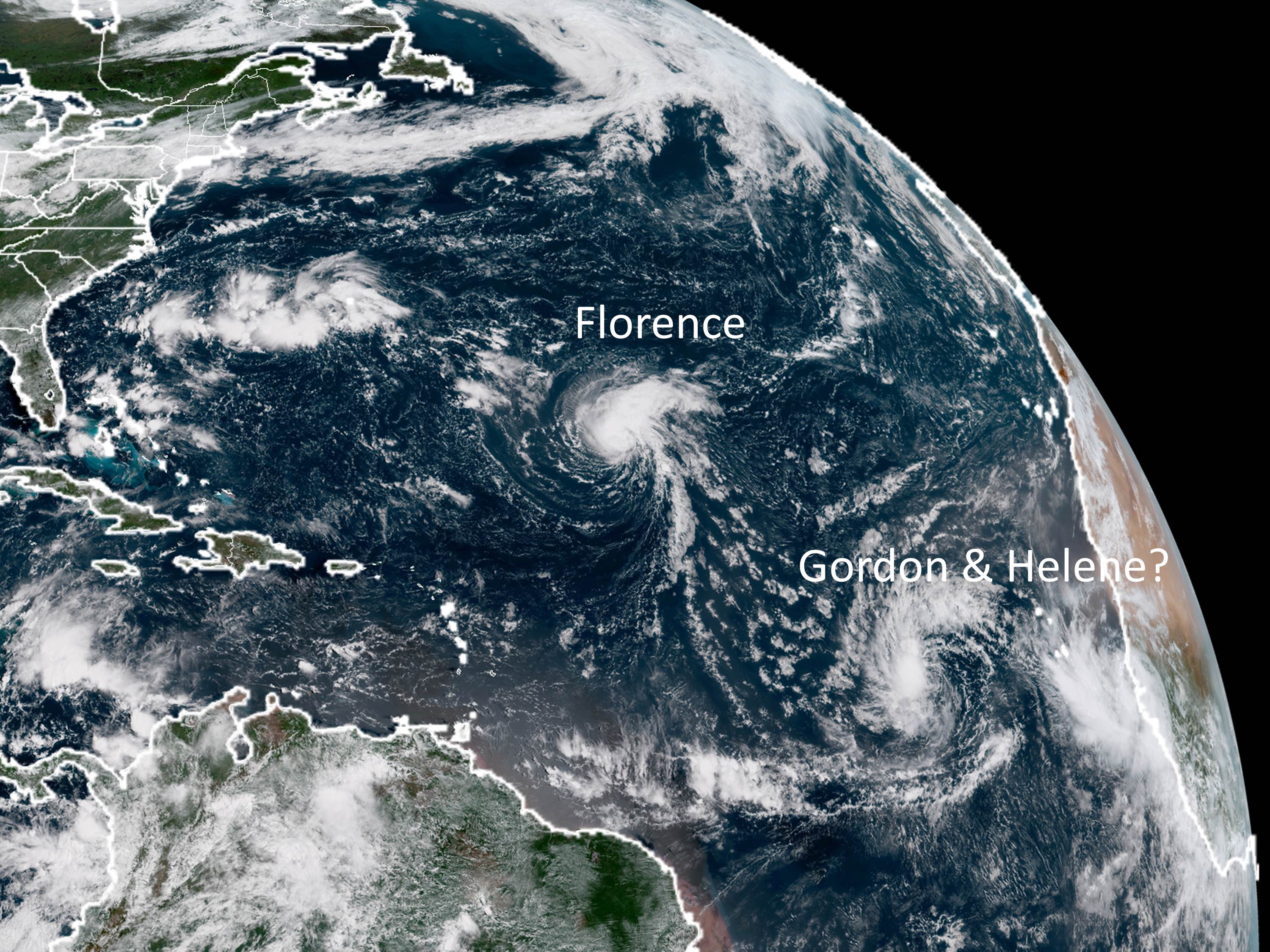
GOES-16 view of the North Atlantic, midday September 7, 2018.
Florence is of the most immediate concern. While still about 6 days away, a variety of weather forecast models are beginning to converge in their forecasts for Hurricane Florence to make landfall somewhere between the Carolinas and Delaware. The latest “spaghetti” plot compiled by the South Florida Water Management District shows the model forecast tracks to be clustering along the mid-Atlantic, with the latest (11 a.m. EDT) official NHC forecast represented by the heavy red line:
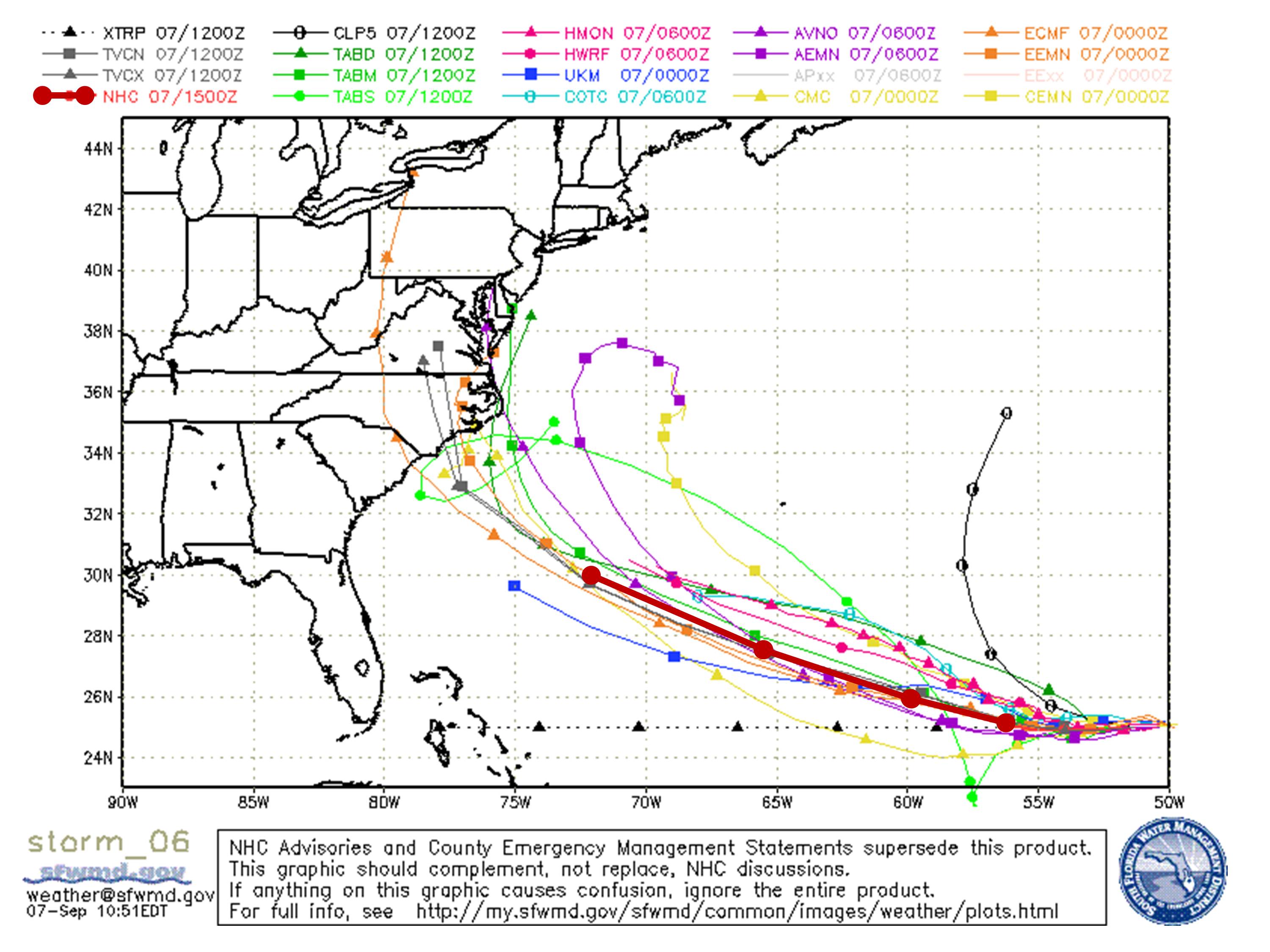
(The westward and northward tracks in the above plot can be ignored.) Florence has temporarily weakened to a strong tropical storm, but should become a hurricane again this weekend, and then a major hurricane (maximum sustained winds of 111 to 130 mph) on Monday or Tuesday.
The two most-watched forecast models are the European ECMWF and the NOAA GFS. Even though it is still too early to place much confidence in their forecasts 6 days out, to give some idea of how those models are treating Florence, here’s this morning’s GFS model bringing Florence inland in North Carolina Thursday morning with wind gusts to 120 mph (graphic courtesy of WeatherBell.com):
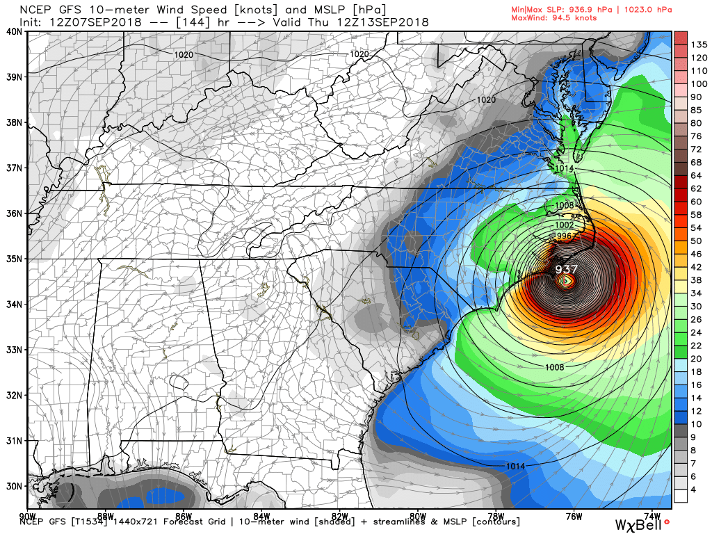
GFS model forecast of Hurricane Florence landfall on the North Carolina coast on Thursday, September 13. This forecast time is still 6 days away, and so likely has a substantial forecast errors.
The GFS then takes Florence up into central Virgina, with 6 to 12 inches of total rainfall mostly east of the track.
The most recent ECMWF model run from last night takes Florence well inland after making landfall near the border of North and South Carolina.
Consistent with the GFS model, Joe Bastardi at Weatherbell.com earlier today predicted the hurricane might track up the Shenandoah Valley, centered on a region already waterlogged from a wet summer, and produce large amounts of additional rainfall the area does not need.
What we know for sure is that large waves and strong rip currents will be a threat along the eastern seaboard this weekend.
Again, it is still too early to place much confidence in any specific forecast. But the trend toward an East Coast landfall is becoming worrisome, and so residents in hurricane-prone areas, especially in the mid-Atlantic states, should be watching the official forecasts from the National Hurricane Center over the next few days in case serious preparations become necessary.