One of the popular (but incorrect) memes of the global warming movement is that storminess is getting worse. While attractive on an emotional level, there is little to no evidence that supports the meme.
Whether it be tornadoes, hurricanes, floods, droughts, or any other class of weather event, there is simply no convincing evidence that any of it is getting worse. Storm damage gets worse over time, of course, as wealth and infrastructure grows (there are more targets for severe weather to strike). But that�s not due to �climate change�.
What people don�t realize is the very large amount of energy which courses through the climate system on a continuous basis which drives all weather and storminess.
Approximately 240 Watts per sq. meter of sunlight is absorbed by the Earth continuously, which equates to 122,000 terajoules (trillion joules) of total energy every second over the entire Earth.
To give that number some perspective, it is the same amount of energy released by all nuclear weapons testing over 50 years�but instead released every 20 seconds.
That�s three times all previous nuclear testing every minute.
180 times all nuclear testing every hour.
4,320 times all nuclear testing every day.
And it�s all entirely normal, occurring whether humans live on Earth or not.
Most of that solar energy is absorbed at the surface of the Earth, which then leads to air currents carrying energy vertically and from one place (where more energy has accumulated) to another (where less energy exists)�especially from the tropics to the polar regions.
Water bodies, especially the oceans, store absorbed solar energy for a period of time, and can release it in large quantities because the near-surface water can overturn, making lots of energy available to the atmosphere.
Because of the orientation of land versus ocean, the spherical nature of the Earth, the Earth�s spin, energy storage by the oceans, and other features of the climate system, it is inevitable that there will be localized large differences in energy content of the atmosphere (which drives all weather) which then results in what we consider a severe weather event. Generally, the greater the temperature difference across a distance, the more the potential energy available for storm formation.
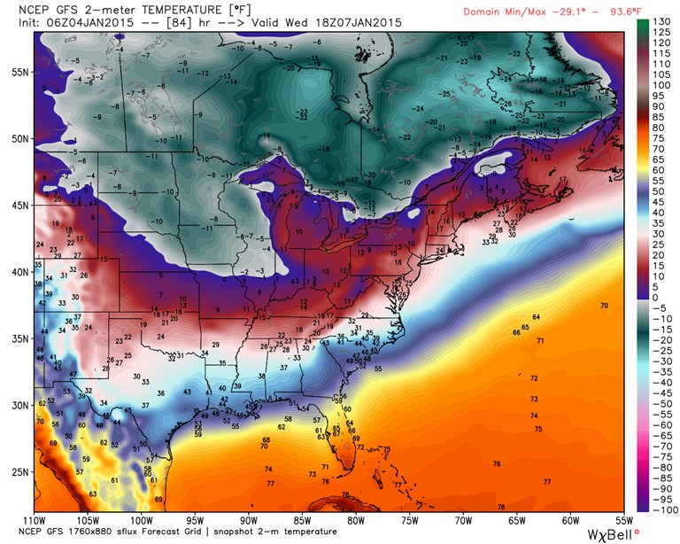
For example, the current surface temperature distribution over Asia exhibits temperature differences of over 150 deg F over a few thousand miles. This type of temperature gradient is what drives, directly or indirectly, almost all storm activity.
It worries me that an increasing portion of the public has the impression that storminess has any significance beyond what has been �normal� for thousands of years. The normal state of weather is to be stormy. Even if humans have caused an overall temperature increase of one degree in the last 50-100 years, it would be difficult to impossible to see such a small change reflected in weather when there is already so much energy available for storm formation. The current energy imbalance of the climate system is theoretically estimated to be about 1%. There is no way — given the chaotic nature of weather — to isolate such a small influence from natural variations.
Even a sunny, cloudless day is the result of storms, the rising air in which forces the air to sink over large regions, creating clear skies. In some sense, those clear skies are a necessary part of the storm circulation. Your sunny day is courtesy of someone else�s story day, hundreds or even thousands of miles away.
The final fate of most of the solar energy which was originally absorbed at the surface as sunlight is then emitted to space by �greenhouse gases� in the atmosphere as infrared radiation. The cycle is complete, and the sun has (for all practical purposes) enough energy to keep the process going forever.
Why am I even bringing this up? Because I saw a news story about some people thinking the localized lake effect snow event in Buffalo last month was due to �climate change�. The claim is so ludicrous that one hardly knows where to start.
Unfortunately, the President’s new initiative to “educate” young people about climate will probably make matters worse, not better.

 Home/Blog