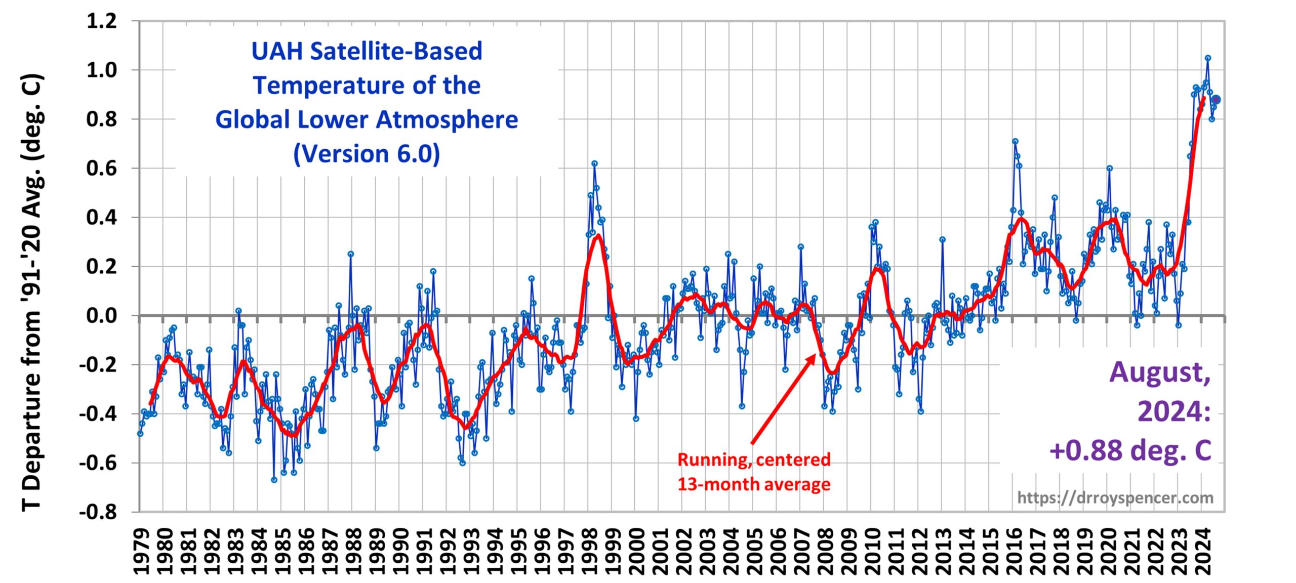
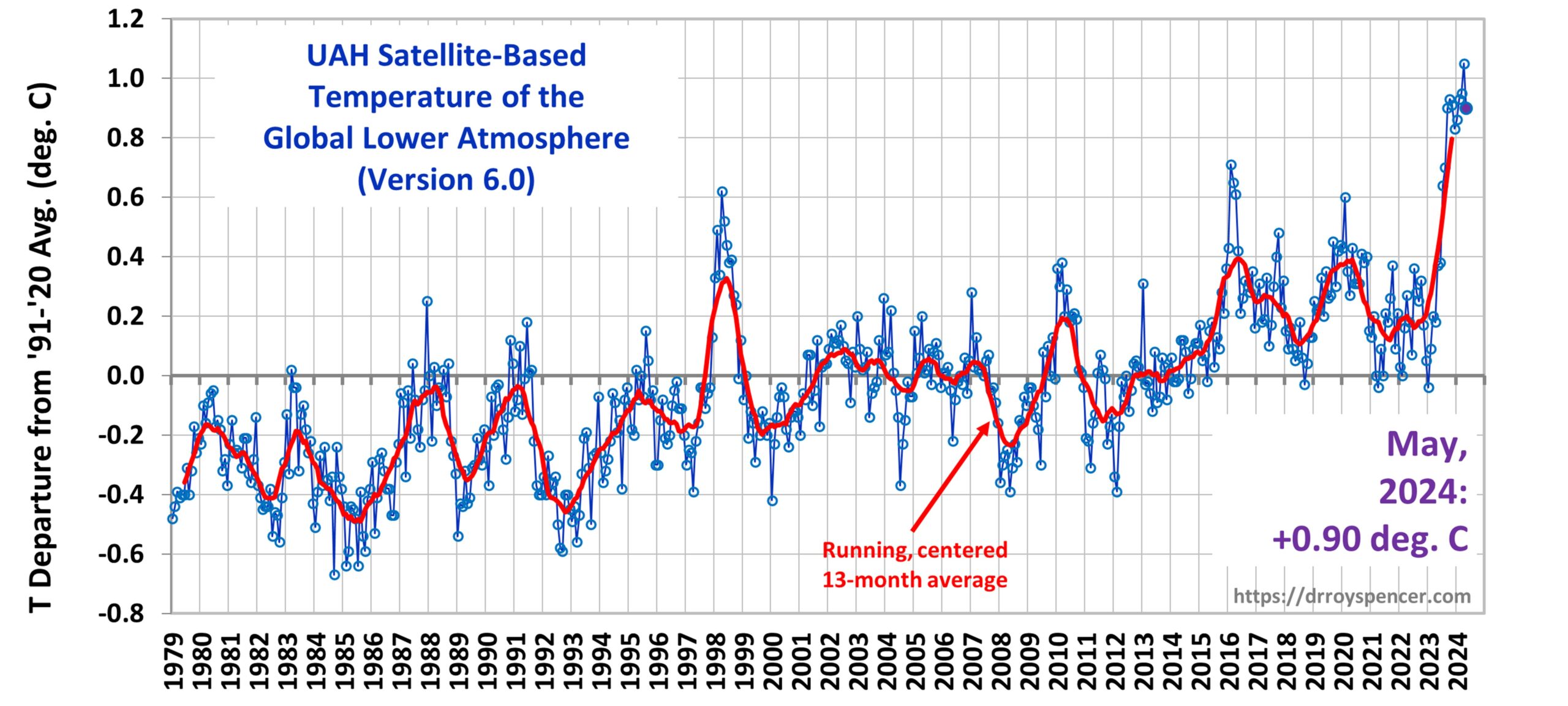
The Version 6 global average lower tropospheric temperature (LT) anomaly for August, 2024 was +0.88 deg. C departure from the 1991-2020 mean, up slightly from the July, 2024 anomaly of +0.85 deg. C.
Persistent global-averaged warmth was (unusually) contributed to this month by the Southern Hemisphere. Of the 27 regions we routinely monitor, 5 of them set record-warm (or near-record) high monthly temperature anomalies in August, all due to contributions from the Southern Hemisphere:
Global land: +1.35 deg. C
Southern Hemisphere land: +1.87 deg. C
Southern Hemisphere extratropical land: +2.23 deg. C
Antarctica: +3.31 deg. C (2nd place, previous record was +3.37 deg. C, Aug. 1996)
Australia: +1.80 deg. C.
The linear warming trend since January, 1979 now stands at +0.16 C/decade (+0.14 C/decade over the global-averaged oceans, and +0.21 C/decade over global-averaged land).
The following table lists various regional LT departures from the 30-year (1991-2020) average for the last 20 months (record highs are in red):
YEAR
MO
GLOBE
NHEM.
SHEM.
TROPIC
USA48
ARCTIC
AUST
2023
Jan
-0.04
+0.05
-0.13
-0.38
+0.12
-0.12
-0.50
2023
Feb
+0.09
+0.17
+0.00
-0.10
+0.68
-0.24
-0.11
2023
Mar
+0.20
+0.24
+0.17
-0.13
-1.43
+0.17
+0.40
2023
Apr
+0.18
+0.11
+0.26
-0.03
-0.37
+0.53
+0.21
2023
May
+0.37
+0.30
+0.44
+0.40
+0.57
+0.66
-0.09
2023
June
+0.38
+0.47
+0.29
+0.55
-0.35
+0.45
+0.07
2023
July
+0.64
+0.73
+0.56
+0.88
+0.53
+0.91
+1.44
2023
Aug
+0.70
+0.88
+0.51
+0.86
+0.94
+1.54
+1.25
2023
Sep
+0.90
+0.94
+0.86
+0.93
+0.40
+1.13
+1.17
2023
Oct
+0.93
+1.02
+0.83
+1.00
+0.99
+0.92
+0.63
2023
Nov
+0.91
+1.01
+0.82
+1.03
+0.65
+1.16
+0.42
2023
Dec
+0.83
+0.93
+0.73
+1.08
+1.26
+0.26
+0.85
2024
Jan
+0.86
+1.06
+0.66
+1.27
-0.05
+0.40
+1.18
2024
Feb
+0.93
+1.03
+0.83
+1.24
+1.36
+0.88
+1.07
2024
Mar
+0.95
+1.02
+0.88
+1.35
+0.23
+1.10
+1.29
2024
Apr
+1.05
+1.25
+0.85
+1.26
+1.02
+0.98
+0.48
2024
May
+0.90
+0.98
+0.83
+1.31
+0.38
+0.38
+0.45
2024
June
+0.80
+0.96
+0.64
+0.93
+1.65
+0.79
+0.87
2024
July
+0.85
+1.02
+0.68
+1.06
+0.77
+0.67
+0.01
2024
August
+0.88
+0.96
+0.81
+0.88
+0.69
+0.94
+1.80
The full UAH Global Temperature Report, along with the LT global gridpoint anomaly image for August, 2024, and a more detailed analysis by John Christy, should be available within the next several days here.
I’ve researched different options regarding commenting with the main intent of reducing bad behavior in the comments section. As many of you know, over the years I’ve banning certain words (which can be circumvented anyway, and inadvertently can lead to acceptable words being banned.)
I’ve also banned certain persons by their IP address, e-mail address, and screen name.
Again, these blocks can all be gotten around, which is why any new commenter must have their first comment be approved by me. This system works pretty well, especially for the few people who cannot hide their identity (think D-C) since their message is always the same.
The biggest problem I’m currently having is that some people who comment here repeatedly belittle others. This does not foster a healthy exchange of ideas, and no one wants to wade through an endless stream of insulting comments.
So, what I am leaning toward is banning of certain individuals who make a habit of insulting others. I will be the sole arbiter of who has crossed the threshold of bad behavior, what constitutes an insult (for a couple of you, it’s a subtle art form), and they will no longer be allowed to post using the same user name, email address, or IP address. This also means that others will not be able to mention them by user name after they are gone, but you all know how to get around that, anyway.
Of course, I cannot prevent those I’ve banned from reappearing with a new user name, email address, and IP address if they are clever enough. But if they resume their bad behavior, they will just be banned all over again. But if they turn over a new leaf… welcome back.
I will not give out warnings regarding bad behavior. Certain people will just disappear from the comments section. Think of me as Big Brother from 1984. Don’t bother protesting, because for each person who is banned I will have a list of quotes from their comments in reserve as evidence.
I will try to remember to post some brief commenting rules at the end of each of my new blog posts so that everyone is forewarned.
As the result of complaints I’m getting regarding certain commenters here who can’t make a point without insulting others, I’ve been forced to read through hundreds of comments. I will probably be implementing one or more changes regarding commenting. More on that later…
I’m also seeing some recurring science talking points that are “incorrect” (as incorrect as can be in the realm of science). I’ve gotten where I’ll let bad science be expressed here if it’s done respectfully, and then let others attempt to correct it. But since not everyone can remember what I’ve blogged on in years past (even I can’t remember some of it), I thought it might be good to review some highlights. It might reduce confusion from some of our newer visitors about what *I* understand and promote from the science, rather than letting my allowing of opinions being expressed here being interpreted as some sort of endorsement of others’ ideas.
Yes, the Greenhouse Effect is like a Real Greenhouse
Most objections to using the greenhouse analogy is that the atmosphere does not have a “roof” preventing convective heat loss like a greenhouse does. But those who claim this don’t realize that the greenhouse effect (GHE) is defined with no convective heat transport. The GHE is like a real greenhouse with a perfect roof. The original paper on this is Manabe & Strickler (1964), where they calculated the average surface temperature in pure radiative equilibrium (the surface and each atmospheric layer achieving a temperature where rates of absorbed and emitted radiation are equal– no convection) was about 70 deg. C warmer than what is actually observed. The weaker “33 deg. C” effect you often see attributed to the GHE is actually the sum of [GHE warming + convective cooling]. It is NOT the extra warming from the GHE alone. So, yes, Virginia, Earth’s greenhouse effect is like a real greenhouse (even more so, because its “roof” is perfect, whereas a real greenhouse roof does lose some heat through conduction of heat through the roof and then convective air currents cooling the roof).
No, the Saturation Effect of Increasing CO2 on Global Temperatures is Not Being Ignored in Global Warming Projections
As CO2 increases in the atmosphere, the effect it has on the loss of IR energy to outer space becomes progressively less, producing a saturation effect. But this is true in all climate models as well, including the ones that produce unrealistic (5 deg. C or more) of warming from a doubling of atmospheric CO2. Thus, invoking the “saturation effect” as a magical talisman to refute CO2-induced warming will not work.
In fact, it is not possible for a planetary atmosphere to become totally opaque to IR radiation, because it would have to be fully, 100% saturated across all pressure-broadening affected wavelengths and through the entire depth of the atmosphere. Even Venus, with ~200,000 times as much CO2 as Earth’s atmosphere, is not “saturated” regarding the absorption of IR radiation.
The saturation talking point seems to have ramped up since publication of the recent theoretical line-by-line computations by my friend Will Happer & his co-author last year. But their calculations result in the same amount of radiative forcing from 2XCO2 as others have computed, and (again) are already included in even the most strongly warming climate models out there. Happer’s calculations might be the most complete and accurate to date (I don’t know), but their results do not change what is already in climate models in any significant way.
Yes, the Cold Atmosphere can Keep the Surface Warmer than if the GHE Did Not Exist
Just like adding insulation to the walls in your house in winter can increase the temperature inside (for the same amount of energy input from a furnace), the “cold” atmosphere helps keep the Earth’s surface warmer than if the radiative insulation it provides did not exist. As I’ve stated before, just take a $50 handheld IR thermometer and point it upward in a clear sky, and see how the indicated temperature warms as you point the thermometer obliquely, away from the zenith. That is the GHE acting on the thermopile within the thermometer, raising its temperature because more IR radiation from the sky occurs from the oblique angle than from pointing it straight up…. even though the atmosphere up there is colder than the interior of the thermometer.
A recent experiment posted at Watts Up With That shows how a cooler object can make a warm object even warmer. Over 10 years ago I used a different experimental setup to demonstrate the same thing.
Now, regarding commenting here… To begin with, I think I will spend a couple of hours computing how many of the frequent commenters’ comments here include insults. Would everyone like to see those statistics? Should we consider an award for the person who has the highest percentage of insults?
As you can tell, Dr. Roy is grumpy this morning.
Now, get off my lawn.
UPDATE:I’m going to start limiting comments to 10 per person per day. Also, at least 50% of some commenters’ comments are just insults or other negative noise with no useful input. Start policing your own behavior because in a week or so I might start posting Insult Scores and banning folks. Others visiting this blog don’t want to wade through all of your negativity to find useful insights.Grumble, grumble…
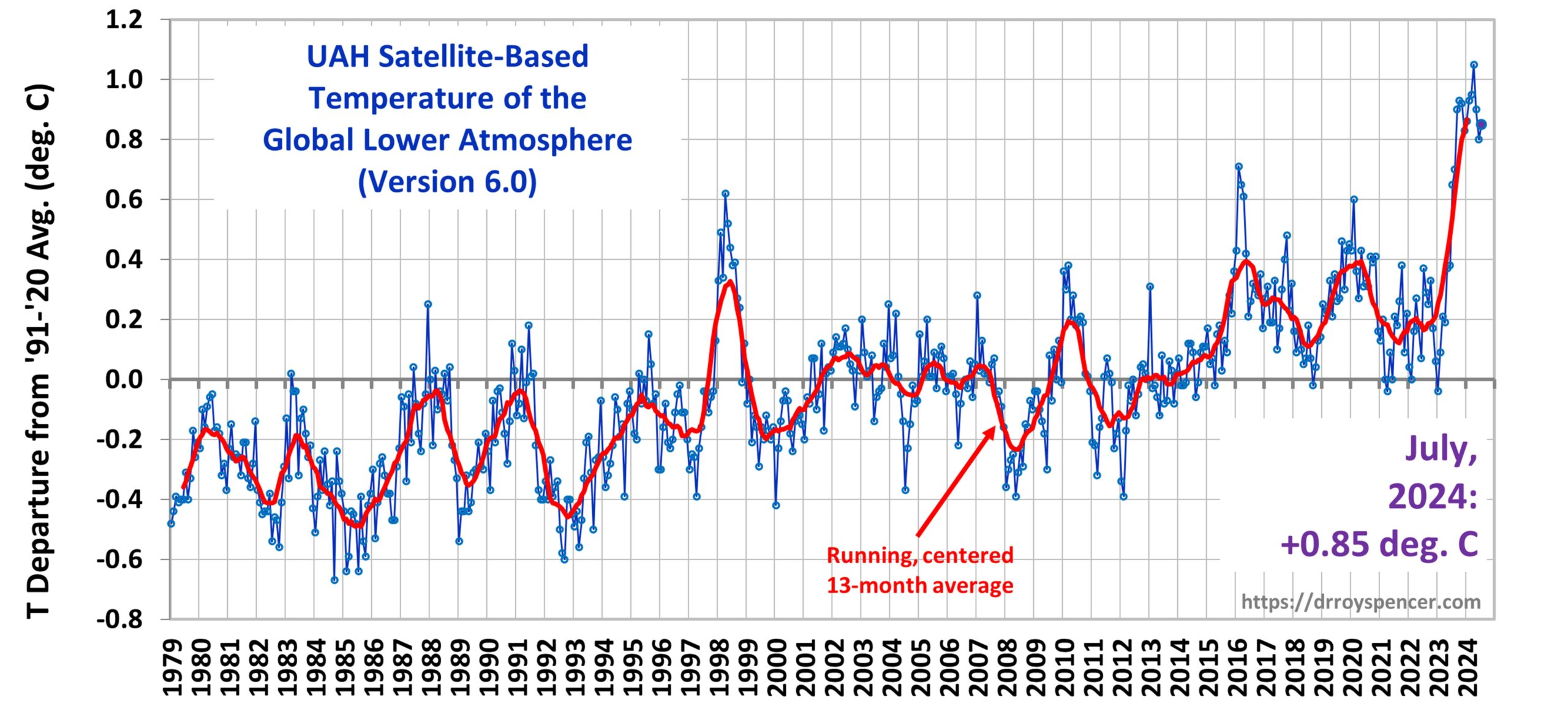
The Version 6 global average lower tropospheric temperature (LT) anomaly for July, 2024 was +0.85 deg. C departure from the 1991-2020 mean, up from the June, 2024 anomaly of +0.80 deg. C.
The linear warming trend since January, 1979 now stands at +0.15 C/decade (+0.13 C/decade over the global-averaged oceans, and +0.21 C/decade over global-averaged land).
The following table lists various regional LT departures from the 30-year (1991-2020) average for the last 19 months (record highs are in red):
YEAR
MO
GLOBE
NHEM.
SHEM.
TROPIC
USA48
ARCTIC
AUST
2023
Jan
-0.04
+0.05
-0.13
-0.38
+0.12
-0.12
-0.50
2023
Feb
+0.09
+0.17
+0.00
-0.10
+0.68
-0.24
-0.11
2023
Mar
+0.20
+0.24
+0.17
-0.13
-1.43
+0.17
+0.40
2023
Apr
+0.18
+0.11
+0.26
-0.03
-0.37
+0.53
+0.21
2023
May
+0.37
+0.30
+0.44
+0.40
+0.57
+0.66
-0.09
2023
June
+0.38
+0.47
+0.29
+0.55
-0.35
+0.45
+0.07
2023
July
+0.64
+0.73
+0.56
+0.88
+0.53
+0.91
+1.44
2023
Aug
+0.70
+0.88
+0.51
+0.86
+0.94
+1.54
+1.25
2023
Sep
+0.90
+0.94
+0.86
+0.93
+0.40
+1.13
+1.17
2023
Oct
+0.93
+1.02
+0.83
+1.00
+0.99
+0.92
+0.63
2023
Nov
+0.91
+1.01
+0.82
+1.03
+0.65
+1.16
+0.42
2023
Dec
+0.83
+0.93
+0.73
+1.08
+1.26
+0.26
+0.85
2024
Jan
+0.86
+1.06
+0.66
+1.27
-0.05
+0.40
+1.18
2024
Feb
+0.93
+1.03
+0.83
+1.24
+1.36
+0.88
+1.07
2024
Mar
+0.95
+1.02
+0.88
+1.35
+0.23
+1.10
+1.29
2024
Apr
+1.05
+1.25
+0.85
+1.26
+1.02
+0.98
+0.48
2024
May
+0.90
+0.98
+0.83
+1.31
+0.38
+0.38
+0.45
2024
June
+0.80
+0.96
+0.64
+0.93
+1.65
+0.79
+0.87
2024
July
+0.85
+1.02
+0.68
+1.06
+0.77
+0.67
+0.01
The full UAH Global Temperature Report, along with the LT global gridpoint anomaly image for July, 2024, and a more detailed analysis by John Christy, should be available within the next several days here.
The monthly anomalies for various regions for the four deep layers we monitor from satellites will be available in the next several days:
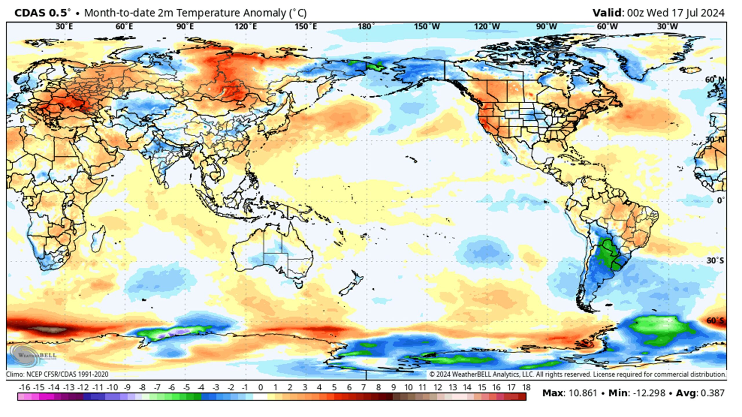
NOAA Climate Data Assimilation System (CDAS) July 2024 surface air temperature departures from 30-year normals, as of July 17, 2024 (graphic courtesy of Weatherbell.com).
That title might trigger some people, so let me explain. Yes, in a warming world due to increasing CO2 there will be a statistical increase in “unusually warm” years. But assuming the warming is entirely due to steadily increasing CO2 causing a slight (currently ~1%) energy imbalance in the climate system, then the warming that results is about ~0.02 deg. C per year.
Anything different from that small 0.02 deg. C per year warming is due to natural climate variability.
This can be easily demonstrated with a simple 1D energy balance model. Anything different is due to natural weather and climate variability.
If we take our UAH global lower tropospheric temperature product as an example, 2023 was a whopping +0.51 deg. C above the 1991-2020 average. Using our trend of +0.14 deg. C per decade as a warming rate baseline, then 2023 should have been +0.25 deg. C above the baseline, but instead it was twice as warm as that. So, about half that warmth was natural (AGAIN… assuming the background warming trend is 100% due to humans).
So, when we get a really warm year (like 2023, and probably 2024) then something other than CO2 is mostly to blame. All of the media and environmentalist hype is just noise. Really warm years will be offset by cooler years (which no one reports on because it’s not newsworthy) so that the long term temperature trends remains ~0.02 deg C per year of warming (+0.014 deg C per year in our satellite data).
Again, this assumes CO2 is 100% to blame for the long-term warming trend, and the 0.02 value assumes a climate sensitivity on the low end of IPCC projections, which is consistent with observations-based diagnoses of climate sensitivity; change it to 0.03 if you want, my point still stands.
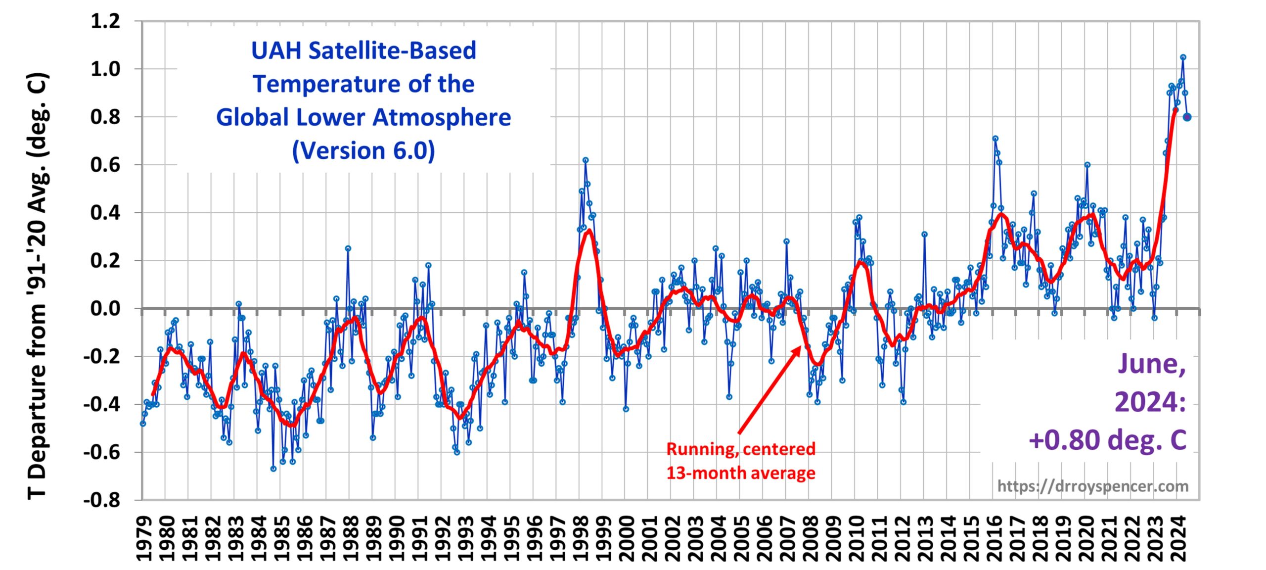
The Version 6 global average lower tropospheric temperature (LT) anomaly for June, 2024 was +0.80 deg. C departure from the 1991-2020 mean, down from the May, 2024 anomaly of +0.90 deg. C.
The linear warming trend since January, 1979 remains at +0.15 C/decade (+0.13 C/decade over the global-averaged oceans, and +0.20 C/decade over global-averaged land).
The following table lists various regional LT departures from the 30-year (1991-2020) average for the last 18 months (record highs are in red):
YEAR
MO
GLOBE
NHEM.
SHEM.
TROPIC
USA48
ARCTIC
AUST
2023
Jan
-0.04
+0.05
-0.13
-0.38
+0.12
-0.12
-0.50
2023
Feb
+0.09
+0.17
+0.00
-0.10
+0.68
-0.24
-0.11
2023
Mar
+0.20
+0.24
+0.17
-0.13
-1.43
+0.17
+0.40
2023
Apr
+0.18
+0.11
+0.26
-0.03
-0.37
+0.53
+0.21
2023
May
+0.37
+0.30
+0.44
+0.40
+0.57
+0.66
-0.09
2023
June
+0.38
+0.47
+0.29
+0.55
-0.35
+0.45
+0.07
2023
July
+0.64
+0.73
+0.56
+0.88
+0.53
+0.91
+1.44
2023
Aug
+0.70
+0.88
+0.51
+0.86
+0.94
+1.54
+1.25
2023
Sep
+0.90
+0.94
+0.86
+0.93
+0.40
+1.13
+1.17
2023
Oct
+0.93
+1.02
+0.83
+1.00
+0.99
+0.92
+0.63
2023
Nov
+0.91
+1.01
+0.82
+1.03
+0.65
+1.16
+0.42
2023
Dec
+0.83
+0.93
+0.73
+1.08
+1.26
+0.26
+0.85
2024
Jan
+0.86
+1.06
+0.66
+1.27
-0.05
+0.40
+1.18
2024
Feb
+0.93
+1.03
+0.83
+1.24
+1.36
+0.88
+1.07
2024
Mar
+0.95
+1.02
+0.88
+1.35
+0.23
+1.10
+1.29
2024
Apr
+1.05
+1.25
+0.85
+1.26
+1.02
+0.98
+0.48
2024
May
+0.90
+0.98
+0.83
+1.31
+0.38
+0.38
+0.45
2024
June
+0.80
+0.96
+0.64
+0.93
+1.65
+0.79
+0.87
The full UAH Global Temperature Report, along with the LT global gridpoint anomaly image for June, 2024, and a more detailed analysis by John Christy, should be available within the next several days here.
The monthly anomalies for various regions for the four deep layers we monitor from satellites will be available in the next several days:
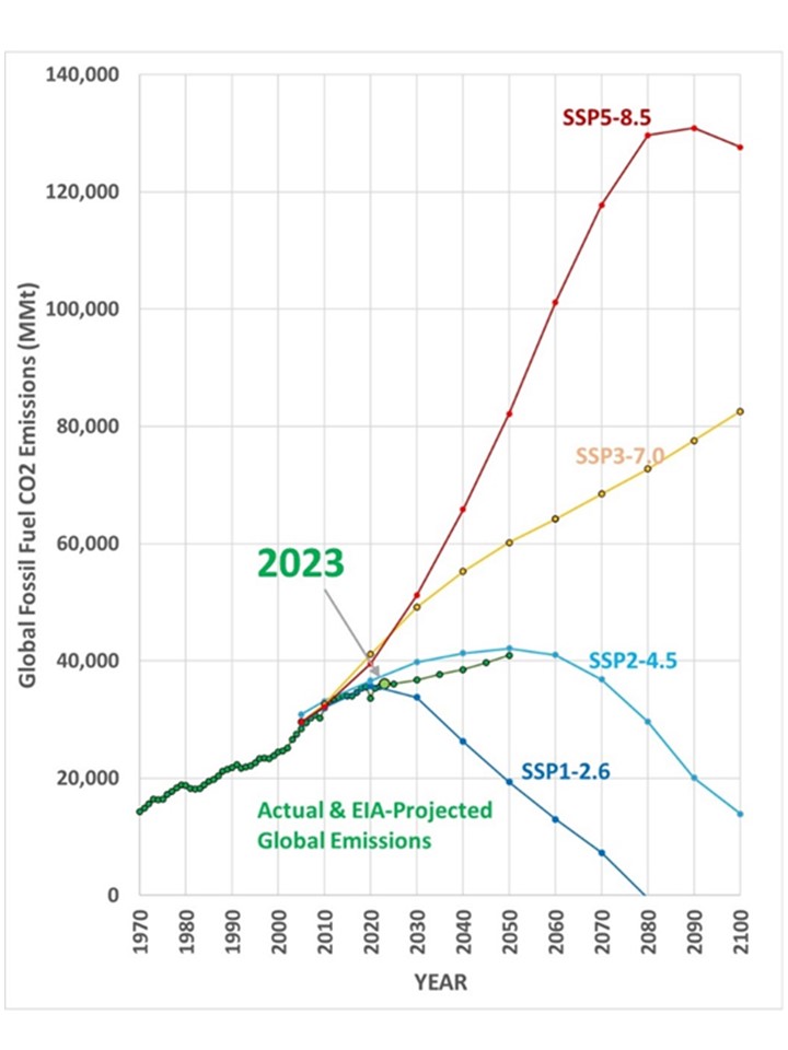
One of the main complaints rational people have had about global warming projections is that the “baseline” scenarios assumed for future CO2 emissions are well above what is realistic. As Roger Pielke, Jr, has been pointing out for years, the U.N. IPCC continues to make these exaggerated scenarios a high priority, and it looks like the next IPCC Assessment Report (AR7) will continue that tradition.
While Roger doesn’t believe there are nefarious motives in this strategy, I do: The IPCC knows very well that as long as climate models are run that produce extreme amounts of climate change, few people will question the assumptions that went into those model projections. Peoples’ careers now depend upon the continuing fear of a “climate crisis” (which has yet to materialize).
But I haven’t been able to find a good, recent graph showing how actual global CO2 emissions compare to those scenarios. So I made one. In the following plot I show estimates of global CO2 emissions from fossil fuel use through 2023, and EIA projections every 5 years from 2025 through 2050 (green). Also shown are the latest (AR6) SSP scenarios that come closest to the AR5 RCP scenarios. (In order to get the SSP scenarios to line up pretty well with the actual emissions in the early years I had to subtract the SSP land use CO2 emissions from the SSP total CO2 emissions values).
While an emissions scenario like SSP5-8.5 has been widely used to scare humanity with climate model projections of extreme warming, this plot shows the last several years of global emissions (through 2023) suggest the future will look nothing like that scenario.
(And, it should come as no surprise that “Net Zero” emissions by 2050 is a delusion.)
I encourage everyone to subscribe to Pielke’s The Honest Broker substack, where he discusses this and related issues in great detail.
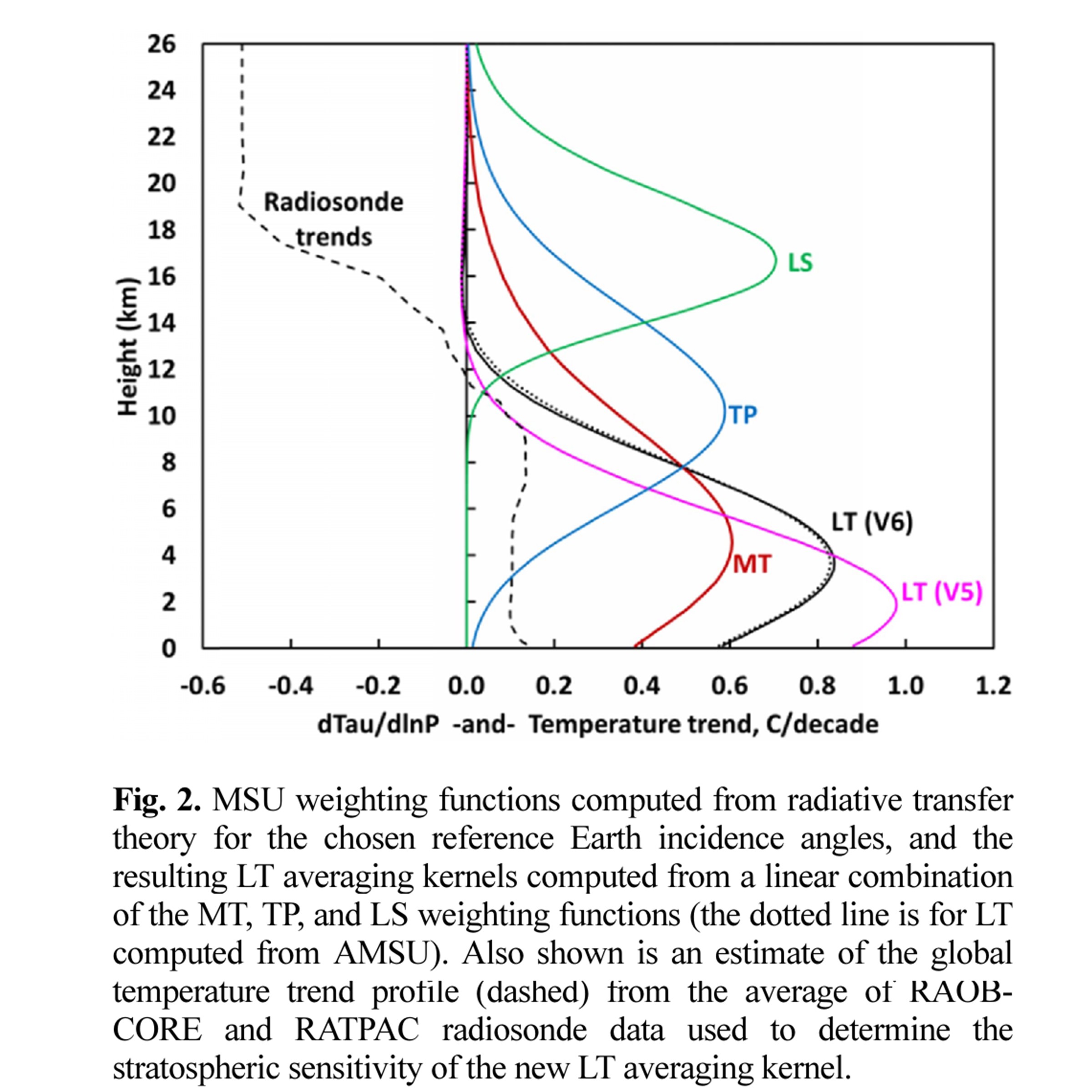
The recent record-setting UAH satellite-based temperatures of the lower troposphere can be compared to a different combination of satellite MSU/AMSU channels which help to corroborate the temperature trends from our “lower tropospheric” (LT) combination of channels.
The three channels we use for LT are MSU channels 2 (“MT”), 3 (“TP”), and 4 (“LS”), (AMSU channels 5, 7, and 9). The primary channel used comes from “MT” (MSU channel 2 or AMSU channel 5), which has the largest weight:
LT = 1.538*MT – 0.548*TP + 0.01*LS
Here is a figure from our 2017 paper on Version 6 of our dataset, showing the three main temperature sounding channels and how they are combined for the LT product:
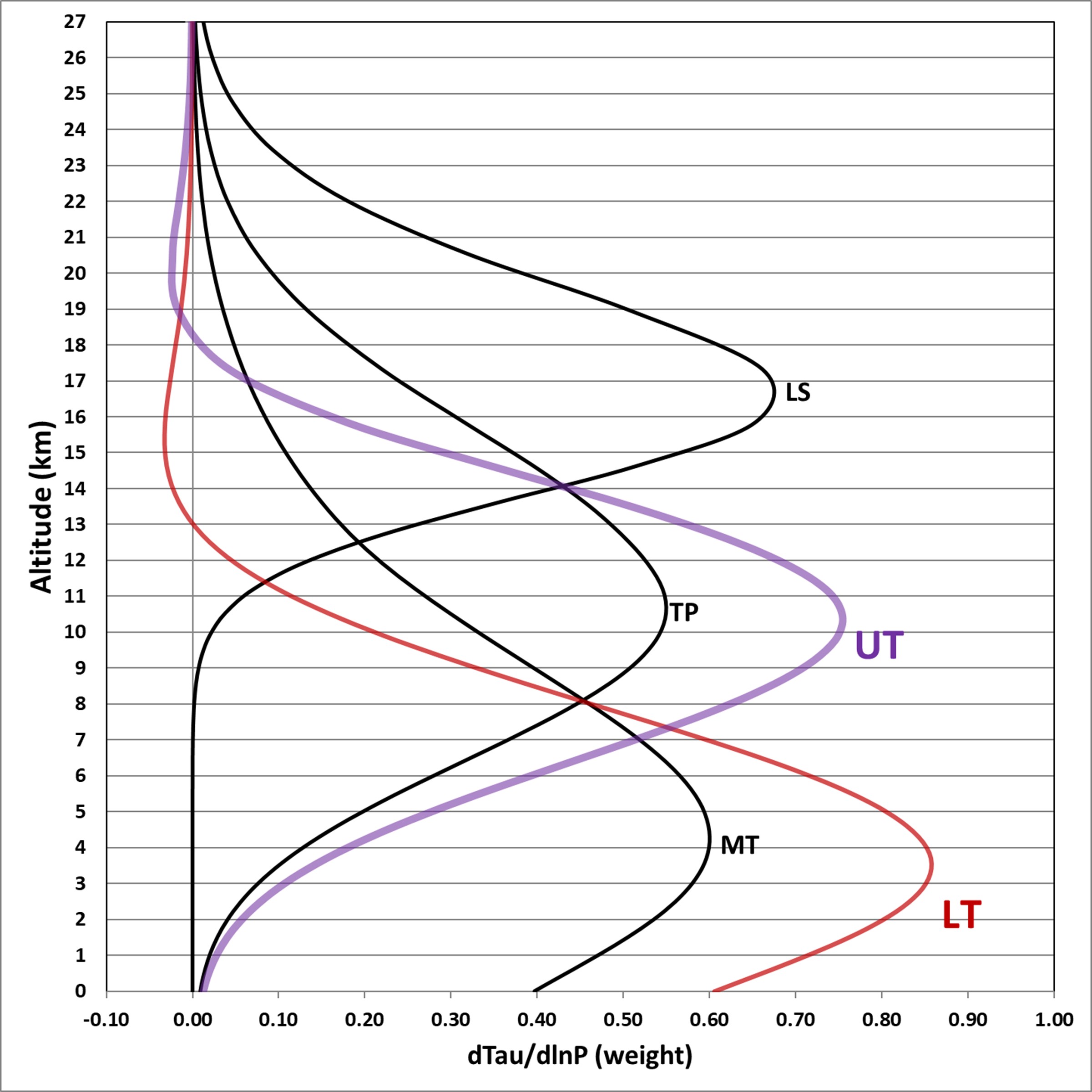
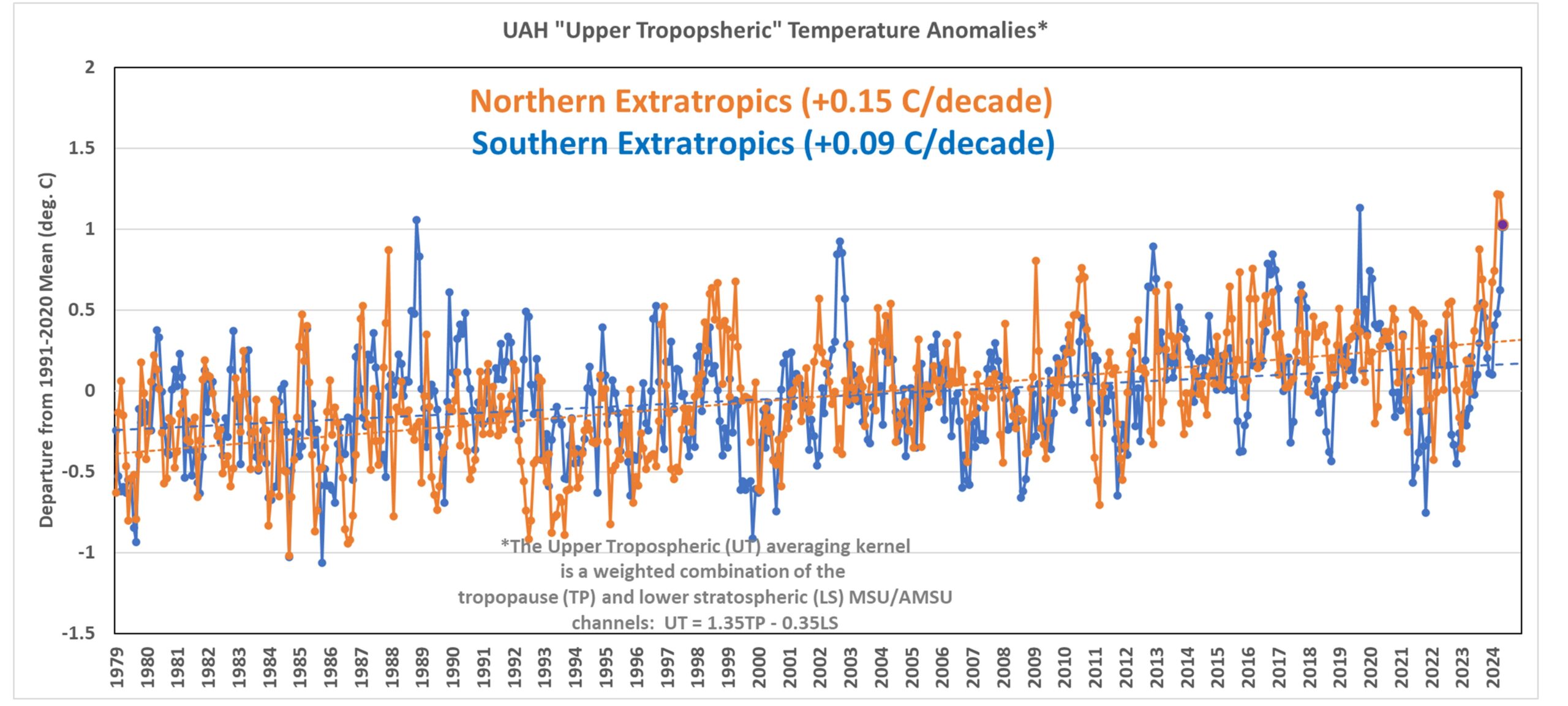
But we have also experimented with a weighted average of MSU channels 3 (“TP”) and 4 (“LS”), (AMSU channels 7 and 9), which produces an averaging kernel in the upper troposphere (nearly insensitive to stratospheric cooling in the tropics, but somewhat sensitive to stratospheric cooling in the extra-tropics where the tropopause [the boundary between troposphere and stratosphere] is lower). This provides an independent check on our LT synthesized channel, keeping in mind one is centered in the lower troposphere and the other is centered in the upper troposphere.
We noticed that last month (May, 2024) produced a record warm global average temperature in the tropopause channel (AMSU channel 7), so I decided to investigate. Combining channel 7 and 9 for an Upper Troposphere (UT) synthesized channel,
UT = 1.35*TP – 0.35*LS
The resulting vertical profile of weight in the atmosphere is the purple curve, below:
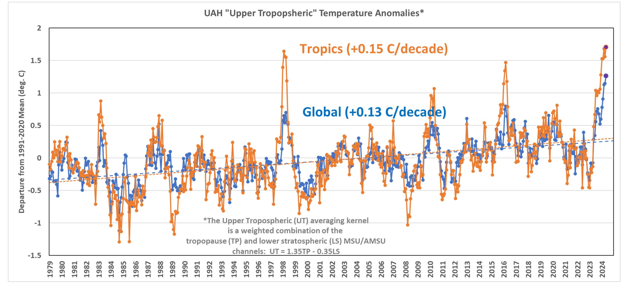
That UT synthesized channel produces the following temperature anomalies:
Note that for the global average, the synthesized UT channel reached record warm values in February, then March, then April, and then May, 2024.
In the tropics, March and then May produced records, but not by much… the 1997/98 El Nino produced upper tropospheric warmth nearly as strong as our recent El Nino.
If we look at just the extra-tropics (next chart) we see the northern latitudes had record warmth in March. But the southern latitudes May came in only 3rd warmest, behind September 2019, and November, 1988.
Note also that the global UT trend is the same as the lower tropospheric (LT) trend, +0.13 C/decade. Since the global UT has some small contamination from lower stratospheric cooling, the “true” UT value (if the stratospheric influence could be removed) would be somewhat warmer. By how much? I’m not sure… maybe +0.15 rather than +0.13 C/decade as an educated guess.
Taken together, I believe this shows that our traditional LT (lower tropospheric) temperature trends are basically corroborated by the other channels of MSU/AMSU.
Keep in mind that when John Christy and I compare these various trends to climate models, it is always apples-to-apples: the climate models’ atmospheric pressure level data are combined and weighted to approximate the same weighting functions as the satellite senses.
The Version 6 global average lower tropospheric temperature (LT) anomaly for May, 2024 was +0.90 deg. C departure from the 1991-2020 mean, down from the record-high April, 2024 anomaly of +1.05 deg. C.
The linear warming trend since January, 1979 remains at +0.15 C/decade (+0.13 C/decade over the global-averaged oceans, and +0.20 C/decade over global-averaged land).
The following table lists various regional LT departures from the 30-year (1991-2020) average for the last 17 months (record highs are in red):
YEAR
MO
GLOBE
NHEM.
SHEM.
TROPIC
USA48
ARCTIC
AUST
2023
Jan
-0.04
+0.05
-0.13
-0.38
+0.12
-0.12
-0.50
2023
Feb
+0.09
+0.17
+0.00
-0.10
+0.68
-0.24
-0.11
2023
Mar
+0.20
+0.24
+0.17
-0.13
-1.43
+0.17
+0.40
2023
Apr
+0.18
+0.11
+0.26
-0.03
-0.37
+0.53
+0.21
2023
May
+0.37
+0.30
+0.44
+0.40
+0.57
+0.66
-0.09
2023
June
+0.38
+0.47
+0.29
+0.55
-0.35
+0.45
+0.07
2023
July
+0.64
+0.73
+0.56
+0.88
+0.53
+0.91
+1.44
2023
Aug
+0.70
+0.88
+0.51
+0.86
+0.94
+1.54
+1.25
2023
Sep
+0.90
+0.94
+0.86
+0.93
+0.40
+1.13
+1.17
2023
Oct
+0.93
+1.02
+0.83
+1.00
+0.99
+0.92
+0.63
2023
Nov
+0.91
+1.01
+0.82
+1.03
+0.65
+1.16
+0.42
2023
Dec
+0.83
+0.93
+0.73
+1.08
+1.26
+0.26
+0.85
2024
Jan
+0.86
+1.06
+0.66
+1.27
-0.05
+0.40
+1.18
2024
Feb
+0.93
+1.03
+0.83
+1.24
+1.36
+0.88
+1.07
2024
Mar
+0.95
+1.02
+0.88
+1.35
+0.23
+1.10
+1.29
2024
Apr
+1.05
+1.25
+0.85
+1.26
+1.02
+0.98
+0.48
2024
May
+0.90
+0.97
+0.83
+1.31
+0.37
+0.38
+0.45
The full UAH Global Temperature Report, along with the LT global gridpoint anomaly image for May, 2024, and a more detailed analysis by John Christy, should be available within the next several days here.
The monthly anomalies for various regions for the four deep layers we monitor from satellites will be available in the next several days:
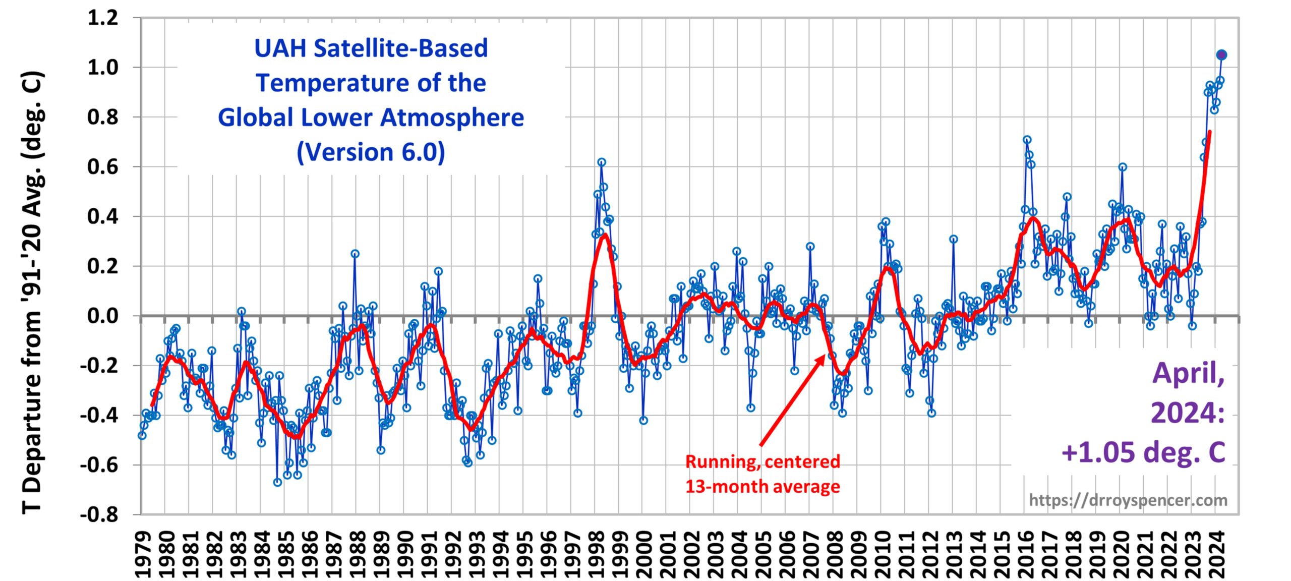
The Version 6 global average lower tropospheric temperature (LT) anomaly for April, 2024 was +1.05 deg. C departure from the 1991-2020 mean, up from the March, 2024 anomaly of +0.95 deg. C, and setting a new high monthly anomaly record for the 1979-2024 satellite period.
The linear warming trend since January, 1979 remains at +0.15 C/decade (+0.13 C/decade over the global-averaged oceans, and +0.20 C/decade over global-averaged land).
It should be noted that the CDAS surface temperature anomaly has been falling in recent months (+0.71, +0.60, +0.53, +0.52 deg. C over the last four months), while the satellite deep-layer atmospheric temperature has been rising. This is usually an indication of extra heat being lost by the surface to the deep-troposphere through convection, and is what is expected due to the waning El Nino event. I suspect next month’s tropospheric temperature will fall as a result.
The following table lists various regional LT departures from the 30-year (1991-2020) average for the last 16 months (record highs are in red):
YEAR
MO
GLOBE
NHEM.
SHEM.
TROPIC
USA48
ARCTIC
AUST
2023
Jan
-0.04
+0.05
-0.13
-0.38
+0.12
-0.12
-0.50
2023
Feb
+0.09
+0.17
+0.00
-0.10
+0.68
-0.24
-0.11
2023
Mar
+0.20
+0.24
+0.17
-0.13
-1.43
+0.17
+0.40
2023
Apr
+0.18
+0.11
+0.26
-0.03
-0.37
+0.53
+0.21
2023
May
+0.37
+0.30
+0.44
+0.40
+0.57
+0.66
-0.09
2023
June
+0.38
+0.47
+0.29
+0.55
-0.35
+0.45
+0.07
2023
July
+0.64
+0.73
+0.56
+0.88
+0.53
+0.91
+1.44
2023
Aug
+0.70
+0.88
+0.51
+0.86
+0.94
+1.54
+1.25
2023
Sep
+0.90
+0.94
+0.86
+0.93
+0.40
+1.13
+1.17
2023
Oct
+0.93
+1.02
+0.83
+1.00
+0.99
+0.92
+0.63
2023
Nov
+0.91
+1.01
+0.82
+1.03
+0.65
+1.16
+0.42
2023
Dec
+0.83
+0.93
+0.73
+1.08
+1.26
+0.26
+0.85
2024
Jan
+0.86
+1.06
+0.66
+1.27
-0.05
+0.40
+1.18
2024
Feb
+0.93
+1.03
+0.83
+1.24
+1.36
+0.88
+1.07
2024
Mar
+0.95
+1.02
+0.88
+1.34
+0.23
+1.10
+1.29
2024
Apr
+1.05
+1.24
+0.85
+1.26
+1.02
+0.98
+0.48
The full UAH Global Temperature Report, along with the LT global gridpoint anomaly image for April, 2024, and a more detailed analysis by John Christy, should be available within the next several days here.
The monthly anomalies for various regions for the four deep layers we monitor from satellites will be available in the next several days:

 Home/Blog